The Telangana Open School Society (TOSS) has officially released the SSC and Intermediate Public Examination Time Table for April/May 2026. Students enrolled under open schooling in Telangana can now prepare according to the confirmed schedule issued by the School Education Department. The examinations will be conducted in accordance with government guidelines and will take place from 20 April 2026 to 27 April 2026 for theory papers.
As per the official notification, theory exams will be held in two separate sessions each day. The morning session is scheduled from 9:00 AM to 12:00 Noon, while the afternoon session will run from 2:30 PM to 5:30 PM. Candidates are advised to report to their examination centres well in advance and carefully check their subject-wise schedule in the detailed annexure provided by TOSS.
In addition to theory examinations, practical exams for eligible SSC and Intermediate subjects will be conducted from 28 April 2026 to 05 May 2026. Students appearing for practical papers should coordinate with their respective study centres for batch-wise timings and instructions.
The release of the TOSS April/May 2026 timetable provides clarity and sufficient preparation time for learners. Students are encouraged to download the official schedule from the TOSS website and begin structured revision to perform confidently in the upcoming public examinations.
TOSS Time Table 2026 Highlights
The Telangana Open School Society (TOSS) has officially announced the SSC and Intermediate Public Examination Time Table for April/May 2026. Students appearing for open school examinations can now plan their preparation as per the confirmed schedule.
Exam Conducting Body: Telangana Open School Society (TOSS)
Examination Levels: SSC & Intermediate
Theory Exam Dates: 20 April 2026 to 27 April 2026
Practical Exam Dates: 28 April 2026 to 05 May 2026
Morning Session Timing: 9:00 AM to 12:00 Noon
Afternoon Session Timing: 2:30 PM to 5:30 PM
Official Notification Date: 19 February 2026
Mode of Examination: Offline (Pen & Paper)
TSOSS Time Table 2026 Important Dates
Day & Date
Course
FN (09:00 AM – 12:00 Noon)
AN (02:30 PM – 05:30 PM)
Day 1 20-04-2026 (Monday)
SSC
Telugu (205), Tamil (237), Oriya (233)
Psychology (222), Marathi (204), Kannada (208)
Inter
Telugu (305), Urdu (306), Hindi (301)
Arabic (310)
Day 2 21-04-2026 (Tuesday)
SSC
English (202)
Indian Culture & Heritage (223)
Inter
English (302)
Sociology (331)
Day 3 22-04-2026 (Wednesday)
SSC
Mathematics (211)
Business Studies (215)
Inter
Political Science (317)
Chemistry (313), Painting (332)
Day 4 24-04-2026 (Friday)
SSC
Science & Technology (212)
Hindi (201)
Inter
Commerce / Business Studies (319)
Physics (312), Psychology (328)
Day 5 25-04-2026 (Saturday)
SSC
Social Studies (213)
Urdu (206)
Inter
History (315)
Mathematics (311), Geography (316)
Day 6 26-04-2026 (Sunday)
SSC
Economics (214)
Home Science (216)
Inter
Economics (318), Mass Communication (335), Biology (314)
Accountancy (320), Home Science (321)
Day 7 27-04-2026 (Monday)
SSC
All Vocational Subjects (Theory 9:00 AM – 11:00 AM; PSTT 9:00 AM – 12:00 Noon)
Intermediate Practical Examinations Dates : 28-04-2026 to 05-05-2026
How to Download TOSS SSC & Inter Time Table 2026
Students can follow these simple steps to download the timetable:
Visit the official website manabadi.co.in.
Navigate to the “TOSS SSC & Inter Time Table 2026” link on the homepage.
Click on the relevant link for SSC or Intermediate.
The timetable PDF will open on the screen.
Download and save the file for future reference.
It is recommended that students take a printout of the timetable and keep it handy for regular reference during exam preparation.
Conclusion
The release of the TOSS SSC & Inter Time Table 2026 at manabadi.co.in has brought relief and clarity to students preparing for the upcoming public examinations. With the detailed schedule now available, candidates can organize their preparation strategy effectively. The timetable serves as a roadmap for students to complete their revision systematically and perform confidently in the exams.
Students are encouraged to stay focused, follow a disciplined study routine, and regularly check official websites for updates. Successfully clearing the TOSS SSC or Intermediate examinations in 2026 will open new academic and career opportunities for learners across Telangana.
The Central Board of Secondary Education (CBSE) has officially issued the CBSE Class 10 Admit Card 2026 for regular candidates on February 2, 2026. Schools can access and download the admit cards through the official portals cbse.gov.in and parikshasangam.cbse.gov.in. Admit cards for private candidates have also been made available online.
Regular students are required to collect their admit cards from their respective schools. Before handing over the document, schools must ensure that the admit card is signed by the school head, and students must sign it along with their parent or guardian. Carrying the admit card on every examination day is compulsory; students without it will not be permitted to appear for the exam.
Private candidates, on the other hand, can download the CBSE 10th admit card 2026 directly from the official website by logging in with their registered credentials.
The Central Board of Secondary Education (CBSE) will conduct the CBSE Class 12 Board Examinations 2026 starting from February 17, 2026. As per the official schedule, the examinations will conclude by April 10, 2026. With the exams approaching, CBSE has announced a significant reform in the evaluation process for Class 12 answer scripts.
CBSE Class 12 Admit Card 2026
CBSE released the CBSE Class 12 Admit Card 2026 on February 2, 2026, through its official website cbse.nic.in. Admit cards for regular students are being downloaded by schools via the CBSE portal. After downloading, schools must ensure that the admit cards are signed by the school principal before distributing them to students.
All Class 12 students are required to collect their admit cards from their respective schools and carry the original copy to the examination centre on every exam day. Entry to the examination hall will be strictly prohibited without a valid admit card.
Private candidates can download their CBSE Class 12 admit card 2026 online using their login credentials from the official website.
CBSE Class 12th Exam 2026 – Overview
Feature
Details
Board
Central Board of Secondary Education (CBSE)
Class
12th (Senior Secondary)
Academic Year
2025–2026
Exam mode
Pen & Paper (Theory) • Practical/Project assessments as per school schedule
Admit Card release
February 2026
Theory exam window
17th Feb – 10th April 2026
Practical exams
Conducted by schools/centers from 1st Jan 2026
Result announcement (expected)
May 2026
Where to download admit card
School distribution / CBSE portal for private candidates / educational portals such as Manabadi
How to Download CBSE Class 12th Admit Card 2026 from manabadi.co.in
While the admit card is officially released on the CBSE academic portal, manabadi.co.in acts as a reliable information platform offering:
TS Inter 1st Year Economics Study Material Textbook Solutions
TS Inter 1st Year Economics Study Material Textbook Solutions are essential for students preparing for the Telangana State Intermediate examinations. These solutions are designed strictly according to the Telangana Board of Intermediate Education (TGBIE) syllabus and help students understand economic concepts in a clear and exam-oriented manner.
Economics is a subject that combines theory, definitions, diagrams, and numerical understanding. With properly structured chapter-wise textbook solutions, students can easily grasp important topics such as Microeconomics, Macroeconomics, Consumer Behaviour, Demand and Supply, National Income, and Economic Growth. Each answer is written in simple language, making it suitable for both average and advanced learners.
The TS Inter 1st Year Economics study material includes detailed explanations, short answers, long answers, and important questions that frequently appear in board exams. These solutions help students write precise and well-structured answers, which is crucial for scoring high marks. Special focus is given to definitions, diagrams, and key points, as they carry significant weight in the evaluation process.
Another major advantage of using Economics textbook solutions is effective revision. Students can revise each chapter quickly before exams without referring to multiple resources. These materials are also helpful for competitive exams and entrance tests, where basic economic concepts are tested.
Students preparing for TS Inter 1st Year Economics exams 2026 can rely on these solutions for accurate content, updated syllabus coverage, and exam-focused preparation. Whether for daily study, revision, or last-minute preparation, TS Inter Economics textbook solutions serve as a complete guide for academic success.
TS Inter 1st Year Economics Study Material in English Medium
Question 1.What are the various definitions of National Income? Describe the determining factors of National Income?
Answer:
National Income has been defined in a number of ways. National income is the total market value of all goods and services produced annually in a country. In other way, the total income accruing to a country from economic activities in a year’s time is called national income. It includes payments made to all factors of production in the form of rent, wages, interest and profits.
The definitions of national income can be divided into two classes. They are : i) traditional definitions advocated by Marshall, Pigou and Fisher, and ii) modern definitions. 1) Marshall’s Definition : According to Alfred Marshall, “the labour and capital of a country acting on its natural resources, produce annually a certain net aggregate of commodities, material and non-material including services of all kinds. This is the true net annual income or revenue of the country”. In this definition, the word ‘net’ refers to deduction of depreciation from the gross national income and to this income from abroad must be added. 2) Pigou’s Definition : According to A. C.Pigou, “National Income is that part of the objective income of the community including of income derived from abroad which can be measured in money”. He has included that income which can be measured in terms of money. This definition is better than the Marshallian definition. 3) Fisher’s Definition : Fisher adopted consumption as the criterion of national income. Marshall and Pigou regarded it as the production. According to Fisher, “the national income consists solely of services as received by ultimate consumers, whether from their material or from their human environment. Only the services rendered during this year are income”. 4) Kuznets’ Definition : From the modem point of view, according to Kuznets, “national income is the net output of commodities and services flowing during the year from the country’s productive system into the hands of the ultimate consumers”. Determining Factors of National income : There are many factors that influence and determine the size of national income in a country. These factors are responsible for the differences in national income of various countries. a) Natural Resources : The availability of natural resources in a country, its climatic conditions, geographical features, fertility of soil, mines and fuel resources etc., influence the size of national income. b) Quality and Quantity of Factors of Production : The national income of a country is largely influenced by the quality and quantity of a country’s stock of factors of production. c) State of Technology : Output and national income are influenced by the level of technical progress achieved by the country. Advanced techniques of production help in optimum utilization of a country’s natural resources. d) Political Will and Stability : Political will and stability in a country helps in planned economic development and for a faster growth of national income.
Question 2.Define national income and explain the various concepts of National Income?
Answer:
National Income means the aggregate value of all the final goods and services produced in the economy in one year. Concepts of National Income : 1) Gross National Product (GNP) : It is the total value of all final goods and services produced in the economy in one year. The main components of GNP are : 1.The goods and services purchased by consumers – C. 2.Investments made by public and private sectors -1. 3.Government expenditure on public utility services – G. 4.Income earned through International Trade (x – m). 5.Net factor income from abroad. GNP at market prices = C + I- G + (x-m)+ Net factor income from abroad. 2) Gross Domestic Product (GDP) : The market value of the total goods and services produced in a country in one particular period usually in a year is the GDP GDP = C + I + G 3) Net National Product (NNP) : Firms use continuously machines and tools for the production of goods and services. This result in a loss of value due to wear and tear of fixed capital. The loss suffered by fixed capital is called depreciation. When we substract depreciation from GNP we get NNP. NNP = GNP – depreciation. 4) National Income at Factor Cost : The cost of production of a good is equal to the rewards paid to the factors which participated in the production process. So the cost of production of a firm is the rent paid on land, wages paid to labour, interest paid on capital and profits of the entrepreneur. National Income at factor cost = NNP + Subsidies – Indirect Taxes – Profits of Govt, owned firms. 5) Personal Income : It is the total of incomes received by all persons from all sources in a specific time period. Personal income is not equal to National Income. Because social security payments. Corporate taxes, undistributed profits are deducted from national income and only the remaining is received by persons. Personal Income = National Income at factor cost – Undistributed profits – Corporate taxes – Social security contributions + Transfer payments. 6) Disposable Income : Personal income totally is not available for spending. Income tax is a payment which must be deducted to obtain disposable income. Disposable Income = Personal income – Personal taxes D.I = Consumption + Savings 7) Per Capita Income : National Income when divided by country’s population, we get per capita income.
The average standard of living of a country is indicated by per capita income.
Question 3.What are the various methods of calculating national income? Explain them. [Mar.’17,’16]
Answer:
There are three methods of measuring National Income. 1.Output method or Product method. 2.Expenditure method. 3.Income method. ‘Carin cross’ says, National Income can be looked in any one of the three ways. As the national income measured by adding up everybody’s income by adding up everybody’s output and by adding up the value of all things that people buy and adding in their savings.
1) Output Method (Product Method) : The market value of total goods and services produced in an economy in a year is considered for estimating National Income. In order to arrive at the value of the product services, the total goods and services produced are multiplied with their market prices. Then, National Income = (P1Q1 + P2Q2 + …. PnQn) – Depreciation – Indirect taxes + Net income from abroad. Where P = Price Q = Quantity 1, 2, 3 n = Commodities & Services There is a possibility of double counting. Care must be taken to avoid this. Only final goods and services are taken to compute National Income but not the raw materials or intermediary goods. Estimation of the National Income through this method will indicate the contribution of different sectors, the growth trends in each sector and the sectors which are lagging behind. 2) Expenditure Method : In this method, we add the personal consumption expenditure of households, expenditure of the firms, government purchase of goods and services net exports plus net income from abroad. NI = EH + EF + EG + Net exports + Net income from abroad. Here, National Income = Private final consumption expenditure + Government final consumption expenditure + Net domestic capital formation + Net exports + Net income from abroad EH = Expenditure of households EF = Expenditure of firms EG = Expenditure of Government Care should be taken to include spending or expenditure made on final goods and services only. 3) Income Method : In this method, the income earned by all factors of production is aggregated to arrive at the National Income of a country. The four factors of production receives income in the form of wages, rent, interest and profits. This is also national income at factor cost. NI = W + I + R + P + Net income from abroad Where, NI = National income W = Wages I = Interest R = Rent P = Profits This method gives us National Income according to distribution of shares.
Short Answer Questions
Question 1.What are the factors that determine National Income? [Mar. ’17, ’16]
Answer:
National Income is the total market value of all goods and services produced in a country during a given period of time. There are many factors that influence and determine the size of national income of a country. a) Natural Resources : The availability of natural resources in a country, its climatic conditions, geographical features, fertility of soil, mines and fuel resources etc., influence the size of National Income. b) Quality and Quantity of Factors of Production : The national income of a country is largely influenced by the quality and quantity of a country’s stock of factors of production. c) State of Technology : Output and national income are influenced by the level of technical progress achieved by the country. Advanced techniques of production help in optimum utilization of a country’s natural resources. d) Political Will and Stability : Political will and stability in a country helps in planned economic development and for a faster growth of National Income.
Question 2.Explain the differences between gross national product at market prices and gross national product at factor prices.
Answer:
National income is the value of all final goods and services produced in a company in a year. Gross National Product (GNP) : Gross National Product is also known as the gross national product at market prices. Gross national product is the current market value of all final goods and services produced in a country during a year including net income from abroad. The main components of GNP are : a) The goods and services purchased by consumers (consumption – C). b) Gross private domestic investment in capital goods (Investment -I) c) Goods and services consumed by the government (Govt expenditure – G) d) Net incomes earned through International trade (value of exports – value of imports, i.e., X-M). GNP = C + I-G + (X-M). GNP at Factor Cost : Gross national product at factor cost is the sum of the money value produced by and accruing to the various factors of production in a year in a country. GNP at market prices includes wages, rent, interest, dividends, undistributed corporate profits, mixed incomes (profits of unincorporated business), direct taxes, indirect taxes, depreciation and net income from abroad. GNP at factor cost includes all items mentioned above in GNP at market prices less indirect taxes. GNP at market prices is always higher than GNP at factor cost. If there are any subsidies to the producers, then to get GNP at factor cost, subsidies are added to GNP at market prices. GNP at factor cost = GNP at market prices = indirect taxes + subsidies.
Question 3.What are National Income at market prices and National income at factor cost?
Answer:
National Income is the value of all the final goods and services produced in a year of a country. National Product at Market Prices (NNP) : The country’s stock of fixed capital undergoes certain amount of wear and tear in producing goods and services over a period of time. This ‘user cost’ or depreciation or charges for renewals and repairs must be substracted from the GNP at market prices to obtain net national product at market prices. NNP at market prices = GNP at market prices – Depreciation. National Product at Factor Cost : It is aslo called as national income. It is the total income received by the four factors of production in the form of rent, wages, interest and profits in an economy during a year. NNP at market prices is not available for distribution among the factors of production. The amount of indirect taxes (which are included in the prices) are paid by the firms to the government and not to the factors of production. Similarly, the government gives subsidies to firms for production of certain types of goods and services and that part of the production cost is borne by the government. Hence, the goods are sold in the market at a lover price than the actual cost of production. Therefore, this volume of subsidies has to broded to the net national income at market prices. Thus, NNP at factor cost = NNP at market prices – Indirect taxes + Subsidies. In another way, NNP at factor cost = GNP at market prices – Depreciation – Indirect taxes + Subsidies.
Question 4.Discuss the three definitions of National Income?
Answer:
National Income has been defined in a number of ways. National income is the toted market value of all goods and services produced annually in a country. In other way, the total income accruing to a country from economic activities in a year’s time is called national income. It includes payments made to all factors of production in the form of rent, wages, interest and profits. The definitions of national income can be divided into two classes. They are : i) traditional definitions advocated by Marshall Pigou and Fisher, and ii) modem definitions. 1) Marshall’s Definition : According to Alfred Marshall, “the labour and capital of a country acting on its natural resources, produce annually a certain net aggregate of commodities, material and non-material including services of all kinds. This is the true net annual income or revenue of the country”. In this definition, the word ‘net’ refers to deduction of depreciation from the gross national income and to this income from abroad must be added. 2) Pigou’s Definition : According to A.C.Pigou, “National Income is that part of the objective income of the community including of income derived from abroad which can be measured in money”. He has included that income which can be measured in terms of money. This definition is better than the Marshallian definition. 3) Fisher’s Definition : Fisher adopted consumption as the criterion of national income. Marshall and Pigou regared it as the production. According to Fisher, “the national income consists solely of services as received by ultimate consumers, whether from their material or from their human environment. Only the services rendered during this year are income”. Fisher definition is better than that of Marshall and Pigou. Because, Fisher’s definition has considered economic welfare which is depending on consumption and consumption represents standard of living. But the definitions advocated by Marshall, pigou, and Fisher are not flawless. The Marshallian and Pigou’s definitions deal with the reasons for economic welfare. But Fisher’s definition is useful to compare economic welfare in different years.
Question 5.How the per capita income is calculated? What is the relationship between population and per capita income?
Answer:
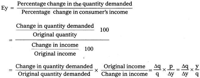
The per capita income is the average income of the people in a country in a particular year. It is calculated by dividing national income at current prices by population of the country in that year. Img1 This refers to the measurement of per capita income at current prices. This concept is a good indicator of the average income and the standard of living in a country. But it is not reliable because actual income may be more or may be less when compared to the average income. This per capita income will also be measured at constant prices and so we get real per capita income. By dividing real national income in a particular year by population of that year we will get real per capita income for that year. Img2 Relationship Between Per Capita Income and Population : There is a close relationship between national income and population. These two together determine the per capita income. If rate of growth of national income is 6% and rate of growth of population is 3% the rate of growth of per capita income will be 3% and it can be expressed as follows : gpc = gni – gp where, gpc = Growth rate of per capita income gni = Growth rate of national income gp = Growth rate of population A rise in the per capita income indicates a rise in standard of living. The rise in per capita income is possible only when the rate of growth of population is less than the rate of growth of that national income.
Relationship among National Income Concepts NIA = Net Income from Abroad D = Depreciation ID = Indirect Taxes Sub = Subsidies UP = Undistributed Profits CT = Corporate Taxes TrH = Transfers received by Households PTP = Personal Tax Payments PTP = Gross Domestic Product GDP = Gross National Product In fig. we have presented the relation between the various concepts of national income.
Question 6.Analyse any two methods of measuring National income?
Answer:
There are three methods of measuring National Income. These are : 1.Output method or Product method 2.Income method, and 3.Expenditure method CaimCross says, “National Income can be looked in any one of the three ways, as the national income measured by adding up everybody’s output by adding up everybody’s income and by adding up the value of all things that people buy and adding in their savings.
1) Output Method or Product Method : It is also known as inventory method or commodity service method. In this method we find the the market value of all final goods and services produced in a country in a year. The entire output of fined goods and services are multiplied by their respective market prices to find out the gross national product. GNP = (P1Q1 + P2Q2 + …. PnQn) + Net income from abroad. Where, GNP == gross national product, P = Price of the goods or services Q = Quantity of goods or services produced 1,2, 3 n are the various goods and services produced. The values of the intermediary goods and services should not be included. Only final goods and services should be taken into account. Here, we find out the value of output by the different sectors like agriculture, government, professionals, industry. 2) Income method : In this method, the incomes earned by all factors of production are aggregated to arrive at the National Income of a country. The four factors of production receives income in the form of wages, rent, interest and profits. Incomes in the form of transfer payment is not included in it. This is also known as national income at factor cost. NI = R + W + I + P NI = National income W = Wages R Rent I = Interest P = Profits
Very Short Answer Questions Question 1. What is National Income? Answer: National income is the market value of goods and services produced annually in a country. Question 2. Mention the factors that determine National Income. Answer: There are many factors that influence and determine the size of national income in a country. These factors are responsible for the differences in national income of various countries. a) Natural Resources : The availability of natural resources in a country, its climatic conditions, geographical features, fertility of soil, mines and fuel resources etc., influence the size of national income. b) Quality and Quantity of Factors of Production : The national income of a country is largely influenced by the quality and quantity of a country’s stock of factors of production. For example, the quantity of agricultural production and hence, the size of National income. c) State of Technology : Output and national income are influenced by the level of technical progress achieved by the country. Advanced techniques of production help in optimum utilization of a country’s natural resources. d) Political Will and Stability : Political will and stability in a country helps for planned economic development for a faster growth of national income. Question 3. Explain the concept of GNP (Gross National Product). Answer: It is the total value of all final goods and services produced in the economy in one year. GNP = C + I + G + (x-m) where, C = Consumption I = Gross National Investment G = Government Expenditure X = Exports M = Imports x – m = Net foreign trade.
Question 4.What is Net National Product at factor cost?
Answer:
It is aslo called as national income. It is the total income received by the four factors of production in the form of rent, wages, interest and profits in an economy during a year. NNP at market prices is not available for distribution among the factors of production. The amount of indirect taxes (which are included in the prices) are paid by the firms to the government and not to the factors of production. Similarly, the government gives subsidies to firms for production of certain types of goods and services and that part of the production cost is borne by the government. Hence, the goods are sold in the market at a lower price than the actual cost of production. Therefore, this volume of subsidies has to be added to the net national income at market prices. Thus, NNP at factor cost = NNP at market prices – Indirect taxes + Subsidies. In another way, NNP at factor cost = GNP at market prices – Depreciation-Indirect taxes + Subsidies. Question 5. What is Personal Income? Answer: It is the total of income received by all persons in a year before payment of all direct taxes. The whole of National Income is not availabe to them. Corporate taxes have to be paid by firms. Firms may keep a part of its profits for expansion. Salaried employees may make contributions for social security. Hence, PI = NI(NNP at factor cost) – (Undistributed corporate profits + Corporate taxes + Social security payments) + Transfer earnings Question 6. What are subsidies?
Question 1.Explain critically the marginal productivity theory of distribution?
Answer:
This theory was developed by J.B. Clark. According to this theory, the remuneration of a factor of production will be equal to its marginal productivity. The theory assumes perfect competition in the market for factors of production. In such a market, average cost and marginal cost of each unit of factor of production are the same as they are equal to the price or cost of a factor of production.
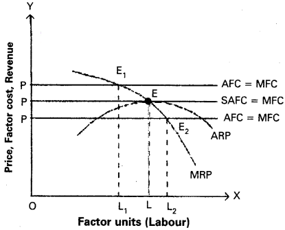
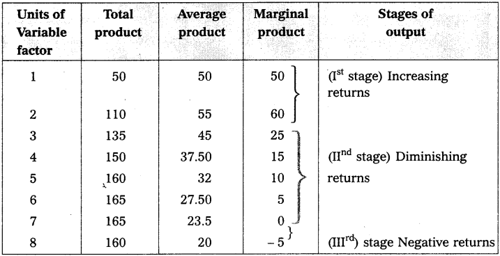
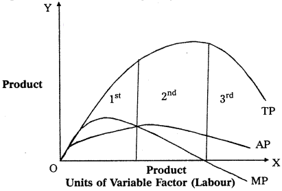
For example, if four tailors can stitch ten shirts in a day and five tailors can stitch thirteen shirts in a day, then the marginal physical product of the 5th tailor is 3 shirts. If stitching charge for a shirt is ₹ 100/-, then the marginal value product of three shirts is ₹ 300/-. According to this theory, the 5th person will be remunerated ₹ 300/-. Marginal physical product is the additional output obtained by using an additional unit of the factor of production. If we multiply the additional output by market price we will get marginal value product or marginal revenue product. At first stage when additional units of labour are employed the marginal productivity of labourer increases up to certain extent due to economies of scale. If additional units’ of labour are employed beyond that point the marginal productivity of labour decreases. This can be shown in the given figure.
In the figure, OX axis represent units of labour and OY represent price/revenue/cost. At a given price, OP the firm will employ OL units of labour where price OP = L. If it employs less than ‘OL’ i.e., OL1 units, MRP will be E1L1, which is higher than the price OR If firm employs more than OL units upto OL2, price is OP is more than E2L2. So the firm decreases employment until price = MRP till OL. At that point ‘E’ the additional unit of labour is remunerated equal to his marginal productivity.
Question 2.Define rent and explain the Ricardian Theory of Rent?
Answer:
David Ricardo was a 19th century economist of England, who propounded a systematic theory of rent. Ricardo defined rent as “that portion of the procedure of earth which is paid to the landlords for the use of the original and indestructible powers of soil”. According to Ricardo, rent arises due to differential in surplus occurring to agriculturists resulting from the differences in fertility of soil of different grades of land.
Ricardian theory of rent is based on the principle of demand and supply. It arises in both extensive and intensive cultivation of land. When land is cultivated extensively, rent on superior land equals the excess of its produce over that of the inferior land. This can be explained with the following illustration.
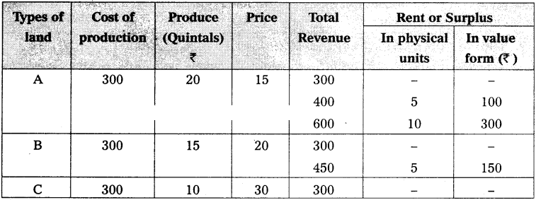
We can imagine that a new island is discovered. Assume a batch of settlers go to that Island. Land in this Island is differ in fertility and situation. We assume that there are three grades of land A, B, and G. With a given application of labour and capital superior lands will yield more output than others. The difference in fertility will bring about differences in the cost of production, on the different grades of land. They first settle on A’ grade land for cultivation of com. A’ grade land yields say, 20 quintals of com with the investment of ₹ 300. The cost of production per quintal is ₹ 15 (300/20). The price of com in the market has to cover the cost of cultivation. Otherwise the farmer will not produce corn. Thus, the price in the present case should be atleast ₹ 15 per quintal.
As time passes, population increases and demand for land also increases. In such a case, people have to cultivate next best land, i.e., ‘B’ grade land. The same amount of ₹ 300 is spent on B’ grade land gives only 15 quintals of com as ‘B’ grade land is less fertile. The cost of cultivation on B’ grade land risen to ₹ 20 (300/15) per quintal of com. If the price of corn per quintal in the market is then ₹ 20, the cultivator of ’B‘ grade land will be not cultivate. Therefore, the price has to be high enough to cover the cost of cultivation on ’B’ grade land. Hence, the price also rises to ₹ 20. There is no surplus on ‘B’ grade land. But on A’ grade land, the surplus is 5 quintals or ₹ 100 (5 × 20).
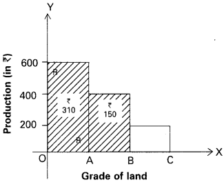
Further, due to growth of population demand for land and corn increased. This necessitates, the cultivation of ‘C’ grade land with ? 300 investment cost. It yields only 10 quintals of com. Therefore, the per quintal production cost rises to 30 (300/10). Then the price per quintal must be atleast ? 30 to cover the cost of production. Otherwise C’ grade land will be withdrawn from cultivation. At price ? 30 C’ grade land yield no surplus or rent. But A grade land yields still layer surplus of 10 quintals or ? 300 (10 x 30). But surplus or rent on ‘B’ grade land has 5 quintals or ? 150 (5 x 30). But there is no surplus or rent on ‘C’ grade land. It covers just the cost of cultivation. Hence, ‘C’ grade land is a marginal land which earns no rent or surplus.This can also be explained with the following table.
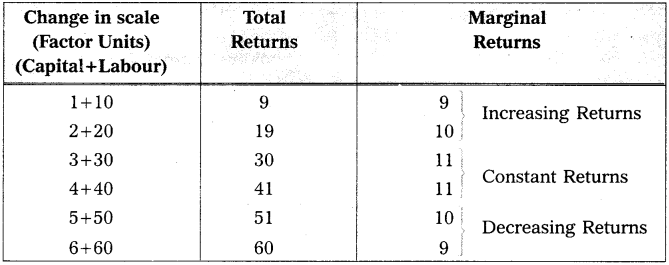
The essence of Ricardian theory of rent.
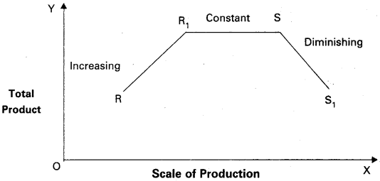
1.Rent is a pure surplus. 2.Rent is differential surplus. 3.Rent does not determine or enter into price. 4.Diminishing returns applies to agricultural production. 5.Land is put to only one use, i.e., for cultivation. Ricardian theory’ of rent can be explained with the help of the above diagram. In the above diagram, the shaded area represents the rent or differential surplus. The least fertile land, i.e., C does not carry any rent. So it is called marginal land or no rent land.
Question 3.What is meant by real wages? What are the factors that determine real wages?
Answer:
The amount of goods and services that can be purchased with the money wages at any particular time is called real wage. Thus, real wage is the amount of purchasing power received by worker through his money wage. Factors Determining the Real Wage :
Methods of Form of Payment : Besides money wages, normally the labourers get some additional facilities provided by their management. Ex : Free housing, free medical facilities etc. As a result, this real wage of the worker will be high.
Purchasing Power of Money : An important factor which determines the real wage is the purchasing power of money which depends upon the general price level. A rise in general price level will mean a full in the purchasing power of money, causes decline in real wages.
Nature of Work : The working conditions also determine the real wages of labourer. Less duration of work, ventilation, fresh air etc., result in high real wages, lack of these facilities then the real wages are low even though if money wages are high.
Future Prospects : Real wage is said to be higher in those jobs where there is possibility of promotions, hike in wages and vice-versa.
Nature of Work : Real wages are also determined by the risk and danger involved in the work. If work is risky wages of labourer will be low though money wages are high. Ex : Captain in a submarine.
Timely Payment : If a labourer receives payment regularly and timely the real wages of the labourer is high although his money wage is pretty less and vice-versa.
Social Prestige : Real wage depends on social prestige. The money wages of Bank officer and judge are equal, but the real wage of a judge is higher than bank officer.
Period and Expenses of Education : Period and expenses of training also affect real wages.
Question 4.Explain about the gross interest and net interest?
Answer:
The concept of interest are two types namely, gross interest and net interest. Gross Interest : The payment which the lender receives from the borrower excluding the principal is gross interest. It comprises the following payments : Net Interest : It is the payment for the service of capital or money only. This is the interest in economic sense. Keynes’ Liquidity Preference Theory : Keynes proposed a monetary explanation of the rate of interest. He said that interest is determined by both the demand for and supply of money. According to J.M. Keynes, “Interest is the reward paid for parting with liquidity for the specified period”. A. Supply of Money : Supply of money refers to the total quantity of money in circulation. Though the supply of money is a function of the rate of interest to a degree, supply of money is fixed or perfectly inelastic at a given point of time. It is determined by the central bank of a country. B. Demand for Money : Keynes coined a new term liquidity preference. People demand money for its liquidity. The desire to hold ready cash is liquidity preference. The higher the liquidity preference, the higher will be the rate of interest to be paid to induce them to part with their liquid assets. The lower the liquidity preference, the lower will be the rate of interest that will be paid to the cash holders. People demand money basically for three reasons : 1) Transactions motive 2) Precautionary motive 3) Speculative motive. 1) Transaction Motive : People desire to keep cash for the current transactions of personal and business exchanges. The amount kept for this purpose depends upon the income and business motives. 2) Precautionary Motive : People keep cash in reserve to meet unforeseen expenses like illness, accidents, unemployment etc. Businessmen keep cash in reserve to gain from unexpected deals in future. Therefore, both individuals and businessmen keep cash in reserve to meet unexpected needs. 3) Speculative Motive : Speculative motive for money relates to the desire to hold cash to take advantage of future changes in the rate of interest and bond prices. The price of bonds and the rate of interest are inversely related. If the prices of bonds are expected to rise then the rate of interest is expected to fall, as businessmen will buy bonds to sell them when their prices rise and vice versa. Low bond prices are indicative of high interest rates, and high bond prices reflect low interest rates.
The demand for money is inversely related to the rate of interest. The transaction and precautionary motives are relatively interest inelastic, but are highly income elastic. In the determination of rate of interest, these two motives do not have any role. Only the speculative motive is interest elastic and this plays very important role in determining the rate of interest with the given supply of money. When the demand for money and supply of money are equal, along with the equilibrium, rate of interest also be determined.
Question 5.What is meant by profit? Explain briefly various theories of profit?
Answer:
Profit is the reward paid to the entrepreneur for his services as an organizer in the process of production. Theories of Profit:
Dynamic theory of profit : This theory was propounded by J.B.Clark. According to Clark, “Profit is the difference between the price and cost of production of commodity”. He viewed that profit as a reward for entrepreneurial dynamism. Dynamic changes like increase in population, new method of production etc., result in increase in profit. In a static economy due to lack of these changes entrepreneurs receive only wages but not profit. Hence, profits are the result of the dynamic changes only.
Innovation theory of profit : This theory was developed by Joseph Schumpeter. According to Schumpeter, “profit is the reward paid to the entrepreneur for his inventive skills”. Because of these inventions profits arise as a difference between prices and costs of production. According to Schumpeter, entrepreneur must break the circular flow by introducing innovations. They are : 1.Introduction of new good. 2.Introduction of new method of production. 3.Reorganisation of industry. 4.Opening up of a new market. 5.Discovery of new source of raw materials. So these innovations, the cost of production remains below its selling price and thus, profit arises. Thus profit is paid to entrepreneur for innovating but not for risk taking.
The risk theory of profit : This theory was proposed by Prof. Hawley. Profits are the reward for an entrepreneur for risk-taking. So the residual part of income after paying all factors of production goes to the entrepreneur for risk taking. Fluctuations in future prices, demand etc., are involved in risk taking. According to Prof. Hawley, “those who face risks in business will be able to earn an excess of payment above the actual value of risk in the form of profit”.
Uncertainty theory of profit : This theory was formulated by Prof. Knight. It is a modified version of risk bearing theory of profits. According to him, profit as the reward for bearing uninsurable risks and uncertainties. He classified risks into two types.
1.Unforeseen insurable risks like fire, theft. 2.Unforeseen non insurable risks like changes in prices, demand and supply. These uninsurable risks cannot be calculated. According to Prof. Knight, “Profit cannot be treated as the reward for risk taking only for reward for uncertainty bearing”.
Walker’s theory of profit : This theory was developed by Walker. According to Walker, “Profits are a rent paid for the abilities of entrepreneur”. Walker theory states that profits arise due to the differences in efficiency and ability of entrepreneurs. Hence, efficient and able entrepreneurs are paid profits.
Short Answer Questions
Question 1.Explain the types of distribution in income?
Answer:
Distribution refers to that branch of economies which analyses how the national income of a community is divided among the various factors of production, distribution then refer to the sharing of the wealth that is produced among factors of production. It is the pricing of factors of production. The distribution of income may be personal or functional. Economies is concerned with functional distribution. The distinction between them is briefly explained here.
Functional Distribution : Functional distribution deals with the study of factor incomes. It means the theory of factor pricing. The prices of land, labour, capital and organisation are called rent, wages, interest and profit respectively. Therefore, it is the study and determination of rent, wages, interest and profit. It concerns the pattern of distribution of national income as rent, wage, interest and profits. Thus, it is not concerned with individuals and their individual income, but with the agents of production. The study of functional shares has been carried on both at the macro and micro levels. Micro-distribution : The theory of micro-distribution explains how the prices of factors of production are determined. Ex : Micro-distribution studies how the wage rate of labour is determined. Macro-distribution : Macro distribution explains the share of a factor of production in the national income. Ex : The share of labour in the national income.
Personal distribution : It refers to the distribution of income or wealth of a country among its people. It studies how income or wealth is distributed among individuals or persons. It studies how much income is earned by an individual, but not how it is earned or in how many forms it is earned. The causes of income inequalities can be known by studying personal distribution.
Question 2.What are the factors that determine the factor prices?
Answer:
The demand and supply of a factor of production determine its price. The demand for a factor of production depends on the following. 1.It depends on the demand for the goods produced by it. 2.Price of the factor determines its demand. 3.Prices of other factors or co-operative factors determine the demand for a factor. 4.Technological changes determine the demand for a factor. 5.The demand for a factor increases due to increase in its production.
Factors that determine the supply of a factor of production.
1.The size of the population and it’s age composition. 2.Mobility of the factor of production. 3.Efficiency of the factor of production. 4.Geographical conditions. 5.Wage also determines the supply of this factor. 6.Income.
Question 3.Point out the assumptions and limitations of marginal productivity theory?
Answer:
Marginal Physical Product (MPP) is the additional output obtained by using an additional unit of the factor of production. If we multiply the additional output by market price we will get Marginal Value Product (MVP) or Marginal Revenue Product (MRP). MRP is the addition made to total revenue by employing one more unit of factor. The marginal revenue productivity of a factor increases initially with the increase in the units of the factor of production, then reaches to maximum and after that it diminishes and will tend to equal the price of the factor service (average factor cost = AFC). This tendency of diminishing marginal revenue productivity follows from the assumption law of variable proportion. Assumptions of the Theory : The theory is based on the following assumptions : 1.There is perfect competition in the factor market and commodity market. 2.All the units of a factor are homogeneous. 3.The theory assumes full employment of the factors. 4.There is perfect mobility of the factors of production. 5.Substitution is possible between the factors. 6.The entrepreneurs are motivated by the profits. 7.Various units of the factors are divisible. 8.The theory is applicable in the long run. 9.It is based on the law of variable proportions. 10.Marginal production of a factor can be measured. Criticism : The marginal productivity theory of distribution is based on unrealistic assump¬tions. Hence, it has been criticized. 1.There is no perfect competition in the factor market and commodity market. 2.All the factor units are not homogeneous. 3.Factors are not fully employed. 4.Factors are not perfectly mobile. 5.Substitution is not always possible between the factors. 6.Profit motive is not the main motive. 7.All factors are not divisible. 8.This theory is not applicable in the short run. 9.Production is not the result of one factor alone. 10.The sum of factor payments is not equal to the value of product. The marginal productivity theory is not an adequate explanation of the determination of the pricing of factors of production. Inspite of limitations of the theory, it explains the role of productivity in the determination of factor price.
Question 4.What are the determining factors of real wages? [Mar. 17, 16]
Answer:
Real wages refer to the purchasing power of money wages received by the labourer. Real wages are expressed in terms of goods and services that a worker can buy with his money wages. The real wage is said to be high when a labourer obtains larger quantity of goods and services with his money income.
Factors Determining Real Wages : Real wages depend on the following factors : 1) Price Level : Purchasing power of money determines the real wage. Purchasing power of money depends on the price level. If price level is high, purchasing power of money will be low. On the contrary, if price level is low, purchasing power of money will be high. Similarly, given the price level, if money wage is high real wage will also increase and when money wage decreases real wage also decreases. 2) Method of Payment : Besides money wages, labourers get certain additional facilities provided by their management. Like free housing, free medical facilities, free education facilities to children, free transport etc. If such facilities are high, the real wages of labourers will also be high. 3) Regularity of Employment : Real wages depend on the regularity of employment. If the job is permanent, his real wage will be high even though his money wage is low. In case of temporary employment, his real wage will be low though his money wage is high. Thus, certainty of job influences real wages. 4) Nature of Work : Real wages are also determined by the risk and danger involved in the work. If the work is risky real wages of labourer will be low though money wages are high. For instance, a captain in a submarine, miners etc., always face danger and risk. 5) Conditions of Work : The working conditions also determine the real wage of a labourer. Less duration of work, ventilation, light, fresh air, recreation facilities etc., certainly result in the high real wages. If these facilities are lacking, real wages are low even though money wages are high. 6) Subsidiary Earnings : If a labourer earns extra income in addition to his wage, his real wage will be higher. For instance, a government doctor may supplement his earnings by undertaking private practice. 7) Future Prospects : Real wage is said to be higher in those jobs where there is a possibility of promotions, hike in wage and vice-versa. 8) Timely Payment : If a labourer receives payment regularly and timely, the real wage of the labourer is high although his money wage is pretty less and vice versa. 9) Social Prestige : Although money wages of a bank officer and Judge are equal, the real wage of a Judge is higher than the bank officer due to social status. 10) Period and Expenses of Education : Period and expenses of education also affect real wage. For example, if one person is a graduate and the other is an undergraduate who are working as clerks, the real wage of the undergraduate is high because his period of learning and expenses on education are lower than the graduate labourer.
Question 5.Explain the concepts of gross profits?
Answer:
Gross profit is considered as a difference between total revenue and cost of production. The following are the components of gross profit: 1.The rent payable to his own land or buildings includes gross profit. 2.The interest payable to his own business capital. 3.The wage payable to the entrepreneur for his management includes gross profit. 4.Depreciation charges or user cost of production and insurance charges are included in gross profit. Net profits : Net profits are reward paid for the organiser’s entrepreneurial skills. Components :
Reward for Risk Bearing : Net profit is the reward for bearing uninsurable risks and uncertainties.
Reward for Co-ordination : It is the reward paid for co-ordinating the factors of production in right proportion in the process of production.
Reward for Marketing Services : It is the profit paid to the entrepreneur for his ability to purchase the services of factors of production.
Reward for Innovations : It is the reward paid for innovations of new products and alternative uses to natural resources.
Wind Fall Gains : These gains arise as a result of natural calamities, wars and artificial scarcity are also included in net profits.
Very Short Answer Questions
Question 1.What are the determining factors of the demand for a factor?
Answer:
1.The demand for the factors of production is derived demand. It depends on the demand for the goods produced by it. 2.Price of the factor determines its demand. 3.Prices of other factors which will help in the production also determine the demand for a factor. 4.Technology determines the demand for the factors. For instance, increase in technology reduces the demand for labourers. 5.Returns to scale will determine the demand for the factors of production. The demand for the factors increases due to increasing returns in the production.
Question 2.What are the determining factors of the surplus of labour ?
Answer:
Supply of labour depends on : 1.Size of the population and its age composition. 2.Mobility of the factors of production. 3.Efficiency of the factors of production. 4.Geographical conditions will determine the supply of factors of production. 5.Price of the factor determines its supply. 6.The supply of a factor depends on its opportunity cost – the minimum earning which it can earn in the next best alternative use.
Question 3.What is Contract rent?
Answer:
It is the hire charges for any durable good. Ex : Cycle rent, room rent etc. It is a periodic payment made for the use of any material good. The amount paid by the tenant cultivator to the landlord annually may be also called contract rent. Ex. : The rent that a tenant pays to the house owner monthly as per an agreement made earlier or the hiring charges of a cycle ^ 10 per hour is also contract rent.
Question 4.What is Economic rent?
Answer:
The ordinary use of the term ‘rent’ means any periodic payment for the hire of anything such as garriages, buildings etc. Economic rent is the pure rent payable as a reward for utilising the productivity of land. It is derived by subtracting the elements like interest, wages, profits and depreciation from the gross rent or contract rent. To David Ricardo, it is surplus over costs or expenses of cultivation.
Question 5.What are Money wages?
Answer:
Money wages are the remuneration received by the labourer in the form of money for the physical and mental service rendered by him or her in the production process. Ex : If a labourer is paid ₹ 30/- per day. ₹ 30/- is the money wage.
Question 6.What are Real wages?
Answer:
Real wage is the purchasing power of money wages in terms of goods and services.
Question 7.What are Time wages?
Answer:
Time wage is the amount paid for labourers for a fixed period of work i.e., weakly, daily, monthly etc.
Question 8.
What are Piece wages?
Answer:
Piece wage is the amount paid for labourers according to volume of work, done by them.
Question 9.
What is Gross interest?
Answer:
The payment which the lender receives from the borrower excluding the principal is gross interest. Gross interest = Net interest + [Reward for risk taking + Reward for Inconvenience + Reward for management]
Question 10.What is Net interest?
Answer:
Net interest is the reward for the service of the capital loan. Ex : Net interest paid on government bonds and government loans.
Question 11.What is Gross profit?
Answer:
Gross profit is considered as a difference between total revenue and cost of production. Gross profit = Net profit + [Implicit rent + Implicit wage + Implicit interest + Depreciation charges + Insurance premium]
Question 12.What is Net profit ? [Mar. ’16]
Answer:
Net profit is the reward paid for the organizer’s entrepreneurial skills. Net profit = Gross profit – [Implicit rent + Implicit wage + Implicit interest + Depreciation charges + Insurance premium]
Question 1.Describe the classification of markets?
Answer:
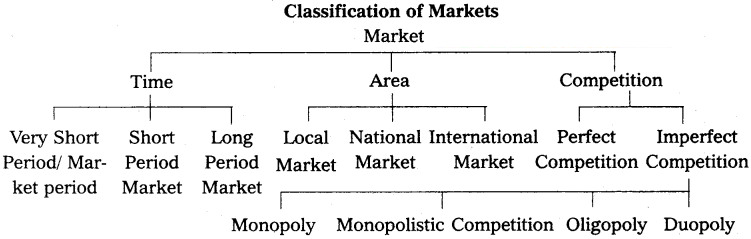
Edwards defined “Market as a mechanism by which buyers and sellers are brought together”. Hence, market means where selling and buying transactions take place. The classification of markets is based on three factors. 1.On the basis of area 2.On the basis of time 3.On the basis of competition.
I. On the Basis of Area : According to the area, markets can be of three types. 1) Local Market : When a commodity is sold at particular locality. It is called a local market. Ex : Vegetables, flowers, fruits etc. 2) National Market : When a commodity is demanded and supplied throughout the country is called national market. Ex : Wheat, rice etc. 3) International Market : When a commodity is demanded and supplied all over the world is called international market. Ex : Gold, silver etc.
II. On the Basis of Time : It can be further classified into three types. 1) Market Period or Very Short Period : In this period where producer cannot make any changes in supply of a commodity. Here, supply remains constant. Ex: Perishable goods. 2) Short Period : In this period supply can be changed to some extent by changing the variable factors of production. 3) Long Period : In this period supply can be adjusted in accordance with change in demand. In long run all factors will become variable.
III. On the Basis of Competition : This can be classified into two types. 1) Perfect Market : A perfect market is one in which the number of buyers and sellers is very large, all engaged in buying and selling a homogeneous products without any restrictions. 2) Imperfect Market : In this market, competition is imperfect among the buyers and sellers. These markets are divided into 1. Monopoly 2. Duopoly 3. Oligopoly 4. Monopolistic competition.
Question 2.What are the characteristic features of perfect competition?
Answer:
Perfect competitive market is one in which the number of buyers and sellers is very large, all engaged in buying and selling a homogeneous products without any restrictions.
The following are the features of perfect competition :
1) Large Number of Buyers and Sellers : Under perfect competition, the number of buyers and sellers is large. The share of each seller and buyer in total supply or total demand is small. So, no buyer and seller cannot influence the price. The price is determined only by demand and supply. Thus, the firm is price taker. 2) Homogeneous Product : The commodities produced by all the firms of an industry are homogeneous or identical. The cross elasticity of products of sellers is infinite. As a result, single price will rule in the industry. 3) Free Entry and Exit : In this competition there is a freedom of free entry and exit. If existing firms are getting profits new firms enter into the market. But when a firm gets losses, it would leave the market. 4) Perfect Mobility of Factors of Production : Under perfect competition the factors of production are freely mobile between the firms. This is useful for free entry and exit of firms. 5) Absence of Transport Cost : There are no transport cost. Due to this, price of the commodity will be the same throughout the market. 6) Perfect Knowledge of the Economy : All the buyers and sellers have full information regarding the prevailing and future prices and availability of the commodity. Information regarding market conditions is also available.
Question 3.Explain the meaning of perfect competition. Illustrate the mechanism of price determination under perfect competition. [Mar. ’17, ’16]
Answer:
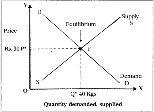
Perfect Competition : Perfect competition is a market sructure characterized by a complete absence of rivalry among the individual firms. Thus, perfect competition in economic theory has a meaning diametrically opposite to the everyday use of this term. In practice, businessmen use the word competition as synonymous to rivalry. In the theory, perfect competition implies no rivalry among firms. Perfect competition may be defined as that market situation, in which there are large number of firms producing homogeneous product, there is free entry and free exit, perfect knowledge on the part of buyer, perfect mobility of factors of production and no transportation cost at all. Price Determination under Perfect Competition : Under perfect competition, sellers and buyers cannot decide the price, Industry decides the price of the good. Market brings about a balance between the commodities that come for sale and those demanded by consumers. It means, the forces of supply and demand determine the price of the good. The following schedule and diagram help us to understand changes in supply, demand and equilibrium price.
Demand and Supply Schedule
Price (In Rupees)
Quantity supplied(in KGs)
Quantity Demanded (in KGs)
10
20
60
20
30
50
30
40
40
40
50
30
50
60
20
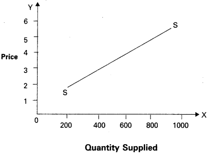
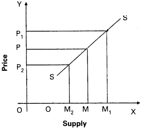
The above table shows the demand and supply schedules of a good. Changes in price always lead to change in supply and demand. As price increases, there is a fall in the quantity demanded. It means, price and quantity demanded have a negative relationship. At the sametime, if price of a commodity increases there is an increase in the quantity supplied. Therefore, the relation between price and supply of goods is positive. It can be observed from the table that when the price is ₹ 10/-, market demand is 60 kgs and supply is 20 kgs.
When the price increases to ₹ 20/-, the supply increases to 30 kgs and demand falls to 50kgs. If the price increases to ₹ 50/-, the supply increases to 60 kgs and demand is only 20 kgs. When the demand is less, price tends to decrease towards equilibrium price. When the price is ₹ 30/-, the demand and supply are equal to 40 kgs. This price is called equilibrium price which is ₹ 30, and equilibrium output and demand is 40 kgs. This process is explained with, the help of figure.
In the figure, the demand and supply of a commodity are shown on OX axis and the price of the commodity on OY axis. As per the diagram, the equilibrium price is found at a point where both demand and supply curves intersect each other at point E, i.e., OP price is the equilibrium price and OQ quantity is the equilibrium supply and demand.
Question 4.Explain equilibrium of the firm in the shortrun and longrun under perfect competition?
Answer:
Perfect competition is a market structure characterized by a complete absence of rivalry among the individual firms. Thus, perfect competition in economic theory has a meaning diametrically opposite to the everyday use of this term. In practice, businessmen use the word competiton as synonymous to rivalry. In theory, perfect competition implies no rivalry among firms. Perfect competition may be defined as that market situation, in which there are large number of firms producing homogeneous product, there is free entry and free exit, perfect knowledge on the part of buyer, perfect mobility of factors of production and no transportation cost at all.
Equilibrium of a Firm : We have learnt that the price of a commodity is determined by the market demand and market supply under perfect competition. An increase in price of a product acts as an incentive in increasing production. As a firm aims at maximizing profit, it chooses that output which maximizes its profits. When the firm is in equilibrium, it has no desire to change its output.
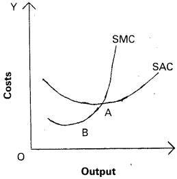
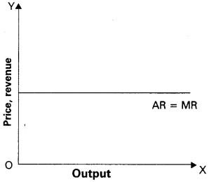
Equilibrium output is explained with the help of cost and revenue curves of a firm. In perfect competition, average and marginal cost curves are ‘U’ shaped one and average revenue and marginal revenue curves are parallel to OX axis. Since AR = MR, both these curves will merge into a single line.
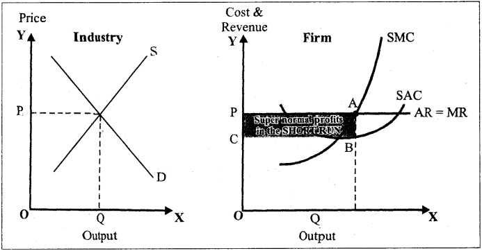
1) Short Period Equilibrium : Firms are in business to maximize profits. During short period, a firm cannot change fixed factors like machinery, buildings etc. However, it produces more output by increasing variable factors. Equilibrium output is produced in the short period where short period marginal cost (SMC) is equal to short period marginal revenue (SMR). The firm will be in equilibrium, when marginal cost curve cuts marginal revenue curve from below. During short period, a firm may get super normal, normal profits or losses. Two conditions are necessary for firm’s equilibrium. They are : i) MC = MR and ii) MC curve should cut MR curve from below. The figure shows the firm’s short period equilibrium.
In the figure quantity demanded and supplied are shown on OX axis and price of the commodity on OY axis. The diagram shows that the equilibrium price OP is determined by the industry at point E where the industry demand is equal to industry supply. The price, so, determined by the industry is passed on to the firm. This is shown by the horizontal demand curve of the firm. This line is also known as the price line. Since, competition is perfect, the AR curve (demand curve) of the firm is also the MR curve of the firm. The firm’s SAC curve and SMC curve are also shown respectively.
The profits of the firm are maximum at the output where MC = MR, that is, at output OQ, SMC = MR. At any output than OQ, MR exceeds MC, which would mean that if the production is more its profits will increase. At any output more than OQ, MR becomes less than MC, which would mean a loss to the firm. Thus, OQ is output of maximum profits. At the equilibrium point ‘E’, the price is equal to OP or AQ, while AC per unit equals QB, profit per unit is equal to B. Total supernormal profits will be equal to PABC, i.e., BA x OQ.
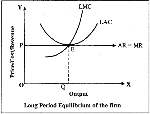
2) Long Period Equilibrium : We have seen that under short period, a firm can adjust its output, within limits, by varying the factors of production. But in the long period the firm can adjust its output to any extent because it can vary all the factors of production. Thus, it is certain that the firm will not incur losses in the long period. In the long period, the free entry of the new firms into the industry will wipe out the supernormal profits of the firm. Hence, in the long period, the frim wil be at optimum size where there is no profit – no loss. Firm gets only normal profits which are included in the long period average cost. In other words, under perfect competition, the individual firm at equilibrium earns normal profits only.
Therefore, AR = MR = LAC = LMC The figure illustrates the long period equilibrium of the firm. The quantity of a good is depicted on OX axis and price, costs and revenues are on OY axis in the diagram.
The point of equilibrium will be established at which the firm’s MR curve touches its LAC curve at its minimum point. At this point LMC = LAC. Thus, when a firm is in long period equilibrium the following conditions exist: At point E; P = AR = MR = LMC = LAC.
Question 5.What is monopoly? Explain how price is determined under monopoly?
Answer:
Monopoly is one of the market in the imperfect competition. The word ‘Mono’ means I ‘single’ and ‘Poly’ means ‘seller’. Thus, monopoly means single seller market. In the words of Bilas, “Monopoly is represented by a market situation in which there is a single seller of a product for which there are no close substitutes, this single seller is unaffected by and does not affect, the prices and outputs of other products sold in the economy”. Monopoly exists under the following conditions : 1) There is a single seller of product. 2) There are no close substitutes. 3) Strong barriers to entry into the industry exist.
Features of Monopoly:
1.There is no single seller in the market. 2.No close substitutes. 3.There is no difference between firm and industry. 4.The monopolist either fix the price or output.
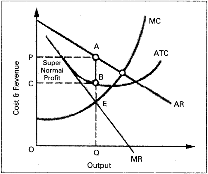
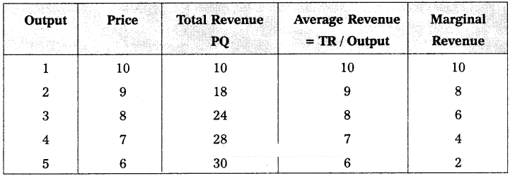
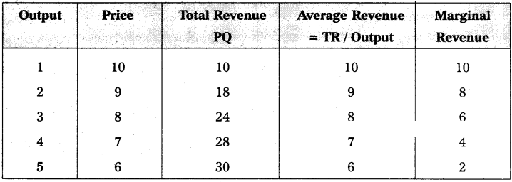
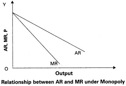
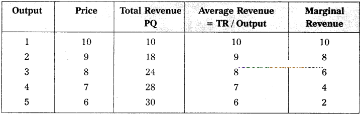
Price Determination : Under monopoly, the monopolist has complete control over the supply of the product. He is price maker who can set the price to attain maximum profit. But he cannot do both things simultaneously. Either he can fix the price and leave the output to be determined by consumer demand at a particular price. Or he can fix the output to be produced and leave the price to be determined by the consumer demand for his product. This can be shown in the diagram.
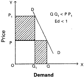
In the above diagram, on ‘OX’ axis measures output and ‘OY axis measures cost. AR is Average Revenue curve, AC is Average Cost curve. In the above diagram, at point E where MC = MR at that point the monopolist determines the output. Price is determined where this output line touches the AR line. In the above diagram for producing OQ quantity cost of production is OCBQ and revenue is OPAQ. Profit = Revenue – Cost = PACB shaded area is profit under monopoly.
Short Answer Questions
Question 1.Write a note on classification of markets based on time and area?
Answer:
Edwards defined, “Market as a mechanism by which buyers and sellers are brought together”. Hence, market means where selling and buying transactions take place. The classification of markets is based on three factors.
1.On the basis of area 2.On the basis of time 3.On the basis of competition. I. On the Basis of Area : According to the area, markets can be of three types. 1) Local Market : When a commodity is sold at particular locality, it is called a local market. Ex : Vegetables, flowers, fruits etc. 2) National Market : When a commodity is demanded and supplied throughout the country is called national market. Ex : Wheat, rice etc. 3) International Market : When a commodity is demanded and supplied all over the world is cdlled international market. Ex : Gold, silver etc. II. On the Basis of Time : It can be further classified into three types. 1) Market Period or Very Short Period : In this period where producer cannot make any changes in supply of a commodity. Here supply remains constant. Ex: Perishable goods. 2) Short Period : In this period supply can be changed to some extent by changing the variable factors of production. 3) Long Period : In this period supply can be adjusted in according to change in demand. In long run all factors will become variable. III. On the Basis of Competition : This can be classified into two types. 1) Perfect market : A perfect market is one in which the number of buyers and sellers is very large, all engaged in buying and selling a homogeneous products without any restrictions. 2) Imperfect Market : In this market, competition is imperfect among the buyers and sellers. These markets are divided into 1. Monopoly 2. Duopoly 3. Oligopoly 4. Monopolistic competition.
Question 2.Explain the equilibrium of the firm in the Short-run under perfect competition?
Answer:
Short Period Equilibrium : Firms are in business to maximize profits. During short period, a firm cannot change fixed factors like machinery, buildings etc. However, it produces more output by increasing variable factors. Equilibrium output is produced in the short period where short period marginal cost (SMC) is equal to short period marginal revenue (SMR). The firm will be in equilibrium, when marginal cost curve cuts marginal revenue curve from below. During short period, a firm may get super normal, normal profits or losses. Two conditions are necessary for firm’s equilibrium. They are : i) MC = MR and ii) MC curve should cut MR curve from below. The figure shows the firm’s short period equilibrium.
In the figure quantity demanded and supplied are shown on OX axis and price of the commodity on OY axis. The diagram shows that the equilibrium price OP is determined by the industry at point E where the industry demand is equal to industry supply. The price, so, determined by the industry is passed on to the firm. This is shown by the horizontal demand curve of the firm. This line is also known as the price line. Since, competition is perfect, the AR curve (demand curve) of the firm is also the MR curve of the firm.
The firm’s SAC curve and SMC curve are also shown respectively. The profits of the firm are maximum at the output where MC = MR, that is, at output OQ, SMC = MR. At any output than OQ, MR exceeds MC, which would mean that if the production is more its profits will increase. At any output more than OQ, MR becomes less than MC, which would mean a loss to the firm. Thus, OQ is output of maximum profits. At the equilibrium point ‘E’, the price is equal to OP or AQ, while AC per unit equals QB, profit per unit is equal to B. Total supernormal profits will be equal to PABC, i.e., BA x OQ.
Question 3.Explain the equilibrium of the firm in the Longrun under perfect competition?
Answer:
Long Period Equilibrium : We have seen that under short period, a firm can adjust its output, within limits, by varying the factors of production. But in the long period the firm can adjust its output to any extent because it can vary all the factors of production. Thus, it is certain that the firm will not incur losses in the long period. In the long period, the free entry of the new firms into the industry will wipe out the supernormal profits of the firm.
Hence, in the long period, the frim wil be at optimum size where there is no profit – no loss. Firm gets only normal profits which are included in the long period average cost. In other words, under perfect competition, the individual firm at equilibrium earns normal profits only. Therefore, AR = MR = LAC = LMC The figure illustrates the long period equilibrium of the firm. The quantity of a good is depicted on OX axis and price, costs and revenues are on OY axis in the diagram. The point of equilibrium will be established at which the firm’s MR curve touches its LAC curve at its minimum point.
At this point LMC = LAC. Thus, when a firm is in long period equilibrium the following conditions exist: At point E; P = AR = MR = LMC = LAC.
Quedtion 4.What is monopoly? What are its characteristics?
Answer:
Monopoly is totally a different market situtation compared with perfect competition. The word ‘mono‘ means single, and ‘poly’ means seller. Monopoly is said to exist when one firm is the sole producer of a product which has no close substitutes. In the words of Bilas, “Monopoly is represented by a market situation in which there is a single seller of a product for which there are no close substitutes, this single seller is unaffected by and does not affect the prices and outputs of other products sold in the economy”.
Characteritics of Monopoly: a) A single firm produces the good in the market. b) No close substitutes to this good. c) Strong barriers exist for the entry of new firms into the market. d) Industry and firm is one and same. e) Producer can control either price or quantity of the good. But he / she cannot determine both price and quantity of the good simultaneously.
Equilibrium and Price Determination under Monopoly : Price, output and profits under monopoly are determined by the forces of demand and supply. The monopolist will have complete control over the supply of the product. He also possesses the power to set the price to attain maximum profit. However, he cannot do both the things simultaneously, Either he can fix the price and leave the output to be determined by the consumer demand at this price or he can fix the output to be produced and leave the price to be determined by the consumer demand for his product.
Question 5.What are the characteristics of monopolistic competition?
Answer:
It is a market with many sellers for a product but the products are different in certain respects. It is mid way of monopoly and perfect competition. Prof. E.H. Chamberlin and Mrs. Joan Robinson pioneered this market analysis.
Characteristics of Monopolistic Competition :
1) Relatively Small Number of Firms : The number of firms in this market are less than that of perfect competition. No one can control the output in the market as a result of high competition. 2) Product Differentiation : One of the features of monopolistic competition is product differentiation. It takes the form of brand names, trade marks etc. Its cross elasticity of demand is very high. 3) Entry and Exit : Entry into the industry is unrestricted. New firms are able to commence production of very close substitutes for the existing brands of the product. 4) Selling Cost : Advertisement or sales promotion technique is the important feature of Monopolistic competition. Such costs are called selling costs. 5) More Elastic Demand : Under this competition the demand curve slopes downwards from left to the right. It is highly elastic.
Question 6.What is oligopoly? Explain its characteristics?
Answer:
The term ‘Oligopoly’ is derived from two Greek word “Oligoi” meaning a few and “Pollein” means to sell. Oligopoly refers to a market situation in which the number of sellers dealing in a homogeneous or differentiated product is small. It is called competition among the few. The main features of oligopoly are the following.
1.Few sellers of the product. 2.There is interdependence in the determination of price. 3.Presence of monopoly power. 4.There is existence of price rigidity. 5.There is excessive selling cost or advertisement cost.
Question 7.Explain the concept of duopoly and its characteristics?
Answer:
Duopoly (from greek duoayi (two) + polein(to sell)) is a specific type of oligopoly where only two producers exist in one market. In reality, this definition is generally used where only two firms have dominance over a market. It is also called as a limited form of oligopoly. The goods produced by the producers may be homogeneous or differentiated. As there are only two producers, both are aware that the decisions of one will affect the other. Rivalry and collusion of the producers are both possible in this market situation. In the market both firms have noteworthy control. In the field of industrial organization, it is the most commonly studied form of oligopoly due to its simplicity.
The earliest duopoly model was developed in 1838 by the French economist Augustin Cournot. Cournot illustrated his model with the example of two firms. According to this model, the two sellers will have a naive behaviours and they never learn from past patterns of reaction of rivalry. As a result each firm produces one third of the output. Together they cover two-thirds of the total market. Each firm maximizes its profits but industry profit will not be maximized. This happens due to non recognition of their interdependence. Characteristics of Duopoly:
a) There will be two sellers. b) Homogeneous product. c) Zero production cost. d) Sellers do not understand their interdependence.
Question 8.Compare perfect Competition and Monopoly?
Answer:
Perfect competition
Monopoly
1. There are large number of sellers.
1. There is only one seller.
2. All products are homogeneous.
2. No close substitutes.
3. There is freedom of free entry and exist.
3. There is no freedom of free entry and exist.
4. There is a difference between the industry and firm.
4. Industry and firm both are same.
5. Industry determines the price and firm receives the price.
5. Firm alone determines the price.
6. There is universal price.
6. Price discrimination is possible.
7. The AR, MR curves are parallel to ‘X’ axis.
7. The AR, MR curves are different and slopes downs from left to right.
Very Short Answer Questions
Question 1.Define Market. [Mar. ’16]
Answer:
Market is place where commodities are brought and sold and where buyers and sellers meet. Communication facilities help us today to purchase and sell without going to the market. All the activities take place is now called as market.
Question 2.Give a note on the Time Based Markets?
Answer:
Supply of a good can be adjusted depending on time factor. On the basis of time, markets are divided into three types, i.e., very short period, short period and long period. a) Market Period or Very Short Period : This is a period where producer cannot make any changes in the supply of a good. Hence, the supply is fixed. As we know supply can be changed by making changes in inputs. Inputs cannot be changed in the very short period. Supply remains constant in this period. Perishable goods will have this kind of markets. b) Short Period : It is a period in which supply can be changed to a little extent. It is possible by changing certain variable inputs like labour. c) Long Period : The market in which the supply can be changed to meet the increased demand, producer can make changes in all inputs depending upon the demand in the long period. It is possible to make adjustments in supply in long period.
Question 3.Give a note on the Area Based Markets?
Answer:
On the basis of area, markets are classified into local, national and international. These markets tell us the size or extent of the market for a commodity. The size of the market for a good depends upon demand for the good, transportation facilities and durability of the good etc. a) Local Market : When a commodity is sold at its produced area it is called local market. Perishable goods like vegetables, flowers, fruits etc., maybe produced and marketed in the same area. b) National Market : When a commodity is demanded and supplied by people throughout the country it is called national market. Examples are wheat, rice, cotton etc. c) International Market : When buying and selling of commodities take place all over the world, then it is called international market. Ex. gold, silver, petrol etc.
Question 4.Give a note on the Competition based markets?
Answer:
Based on the nature of the competition, markets are classified into two perfect competition and imperfect competition. a) Perfect Competition : A perfectly competitive market is one in which the number of buyers and sellers is very large, all engaged in buying and selling a homogeneous product without any artificial restrictions. Hence, there is absence of rivalry among the individual firms in perfect competition. b) Imperfect Competition : It is a market situation where competition is not perfect either amongst the buyers or amongst the sellers. Hence, there will be a different price for the same product. These markets are divided into monopoly, monopolistic competition, oligopoly and duopoly.
Question 5.What is Perfect competition?
Answer:
In this market there are large number of buyers and sellers who promote competition. In this market goods are homogeneous. There is no transport fares and publicity costs. So price is uniform of any market.
Question 6.Define Monopoly?
Answer:
Mono means single, Poly means seller. In this market single seller and there is no close substitutes. The monopolist is a price maker.
Question 7.What is Monopolistic competition? [Mar. ’16]
Answer:
It is a market where several firms produce same commodity with small differences is • called monopolistic competition. In this market producers to produce close substitute goods. Ex : Soaps, cosmetics etc.
Question 8.Define Oligopoly?
Answer:
A market with a small number of producers is called oligopoly. The product may be homogeneous or may be differences. This market exists in automobiles, electricals etc.
Question 9.What is Duopoly?
Answer:
When there are only two sellers of a product, there exist duopoly. Each seller under duopoly must consider the other firms reactions to any changes that he makes in price or output. They make decisions either independently or together.
Question 10.Explain Equilibrium price?
Answer:
Equilibrium price is that price where demand and supply are equal in the market.
Question 11.What is Product differentiation? [Mar. ’17]
Answer:
One of the main features of monopolistic competition is product differentiation. This is a market situation in which there are many firms of a particular product, but the product of each firm is in some way or the other way differentiated from the product of the other firms in the market. They are heterogeneous rather than homogeneous. Product differentiation may take the form of brand names, trademarks, etc. This means that the products of the firms will have close substitutes and their cross-elasticity of demand will be very high.
Question 12.What are the Selling costs? [Mar. ’17]
Answer:
An important feature of a monopolistic market is every firm makes expenditures to sell more output. Advertisements through newspapers, journals, electronic media etc., these methods are used to attract more consumers by each firm.
Question 1Critically examine the law of variable proportions. [Mar. ’16]?
Answer:
The law of variable proportions has been developed by the 19th-century economists David Ricardo and Marshall. The law is associated with the names of these two economists. The law states that by increasing one variable factor and keeping other factors constant, how to change the level of output, total output first increases at an increasing rate, then at a diminishing rate, and later decreases. Hence, this law is also known as the “Law of Diminishing returns”. Marshall stated it in the following words. “An increase in capital and labour applied in the cultivation of land causes, in general, less than proportionate increase in the amount of produce raised, unless it happens to coincide with an improvement in the arts of agriculture”. Assumptions : 1.The state of technology remain constant. 2.The analysis relates to short period. 3.The law assumes labour in homogeneous. 4.Input prices remain unchanged. Explanation of the Law : Suppose a farmer has ‘4’ acres of land he wants to increase output by increasing the number of labourers, keeping other factors constant. The changes in total production, average product and marginal product can be observed in the following table.
In the above table total product refers to the total output produced per unit of time by all the labourers employed. Average product refers to the product per unit of labour marginal product refers to additional product obtained by employing an additional labour.
In the above table there are three stages of production. 1st stage i.e., increasing returns at 2 units total output increases average product increases and marginal product reaches maximum.
2nd stage i.e., diminishing returns from 3rd unit onwards TP increases at diminishing rate and reaches maximum, MP becomes zero and AP continuously decreases. 3rd stage i.e., negative returns from 8th unit TP, decreases AP declines and MP becomes negative. This can be explained in the following diagram.
In the diagram, on ‘OX’ axis shown units labourer and ‘OY axis show TP, MP, and A.P. 1st stage TP AP increases and MP is maximum. In the 2nd stage TP is maximum, AP decreases and MP is zero. At 3rd stage TP declines, AP also declines, MP becomes negative.
Question 2.Explain the law of returns to scale. [Mar. ’17]?
Answer:
The law of returns to scale relate to long run production function. In the long run it is possible to alter the quantities of all the factors of production. If all factors of production are increased in given proportion the total output has to increase in the same proportion. Ex : The amounts of all the factors are doubled, the total output has to be doubled, increasing all factors in the same proportion is increasing the scale of operation. When all inputs are changed in a given proportion, then the output is changed in the same proportion. We have constant returns to scale and finally arises diminishing returns. Hence, as a result of change in the scale of production, total product increases at increasing rate, then at a constant rate and finally at a diminishing rate. Assumptions : 1.All inputs are variable. 2.It assumes that state of technology remains the same. The returns to scale can be shown in the following table.
The above table reveals the three patterns of returns to scale. In the 1st place, when the scale is expanded upto 3 units, the returns are increasing. Later and upto 4th units, it remains constant and finally from 5th onwards the returns go on diminishing.
In the diagram, on ‘OX’ axis shown scale of production, on ‘OY’ axis shown total product. RR1 represents increasing returns R1S – Constant returns; SS1 represents diminishing returns.
Question 3.Describe the internal and external economies?
Answer:
Economies of large scale production can be grouped into two types. 1.Internal economies 2.External economies.
Internal Economies : Internal economies are those which arise from the expansion of the plant, size or from its own growth. These are enjoyed by that firm only. “Internal economies are those which are open to a single factory or a single firm independently of the action of other firms.” – Cairncross i)Technological Economies : The firm may be running many productive establishments. As the size of the productive establishments increase, some mechanical advantages may be obtained. Economies can be obtained from linking process to another process i.e., paper making and pulp making can be combined. It also uses superior techniques and increased specialization. ii) Managerial Economies : Managerial economies arises from specialisation of management and mechanisation of managerial functions. For a large size firm it becomes possible for the management to divide itself into specialised departments under specialised personnel. This increases efficiency of management at all levels. Large firms have the opportunity to use advanced techniques of communication, computers etc. All these things help in saving of time and improve the efficiency of the management. iii) Marketing Economies : The large firm can buy raw materials cheaply, because it buys in bulk. It can secure special concession rates from transport agencies. The product can be advertised better. It will be able to sell better. iv) Financial Economies : A large firm can arise funds more easily and cheaply than a small one. It can borrow from bankers upon better security. v) Risk Bearing Economies : A large firm incurs unrisk and it can also reduce risks. It can spread risks in different ways. It can undertake diversifications of output. It can buy raw materials from several firms. vi) Labour Economies : A big firm employs a large number of workers. Each worker is given the kind of job he is fit for.
External Economies : An external economy is one which is available to all the firms in an industry. External economies are available as an industry grows in size. i) Economies of Concentration : When a number of firms producing an identical product are localised in one place, certain facilities become available to all. Ex : Cheap transport facility, availability of skilled labour etc. ii) Economies of Information : When the number of firms in an industry increases collective action and co-operative effort becomes possible. Research work can be carried on jointly. Scientific journal can be published. There is a possibility for exchange of ideas. iii) Economies of Disintegration : When the number of firms increases, the firm may agree to specialise. They may divide among themselves the type of products of stages of production. Ex : Cotton industry.
Question 4.Explain short-run costs illustrations?
Answer:
Costs are divided into two categories i.e., 1.Short run cost curves 2.Long run cost curves. In short run by increasing only one factor i.e., (labour) and keeping other factor constant. The short run cost are again divided into two types. 1.General costs 2.Economic costs.
General Costs : i) Money Costs : Production is the outcome of the efforts of factors of production like land, labour, capital and organisation. So, rent to land, wage to labour, interest to capital and profits to entrepreneur has to be paid in the form of money is called money cost. ii) Real Cost : Adam Smith regarded pains and sacrifices of labour as real cost. So, it cannot be measured interms of money. iii) Opportunity cost : Factors of production are scarce and have alternative uses. The opportunity cost of a factor is the benefit that is foregone from the next best alternative use.
Economic Costs : i) Fixed Costs : The cost of production which remains constant even when the production may be increased or decreased is known as fixed cost. The amount spent by the cost of plant and equipment, permanent staff are treated as fixed costs. ii) Variable Cost : The cost of production which is changing according to changes in the production is said to be variable cost. In the long period all costs are variable costs. It includes prices of raw materials, payment of fuel, excise taxes etc. Marshall called it as “Prime cost”. iii) Average Cost : Average cost means cost per units of output. If we divided total cost by the number of units produced, we will get average cost.
iv) Marginal Cost : Marginal cost is the additional cost of production producing one more unit. MC = ΔTCΔQ v) Total cost : Total cost is the sum of total fixed cost and total variable cost. TC = FC + VC The short term cost in relation to output are explained with the help of a table.
In the above table shows that as output is increased in the 1st column, fixed cost remains constant. Variable costs have changed as and when there are changes in output. To produce more output in the g TVC short period, more variable factors have to be employed. By adding FC & VC we get total cost at different levels of output. AC falls output increases, reaches its minimum and then rises MC also change in the total cost associated with a change in output. This can be shown in the diagram. In the above diagram is on ‘OX’ axis taken by output and ‘OY axis is taken by costs. The shapes of different cost curves explain the relationship between output and different costs. TFC is horizontal to ‘X’ axis. It indicates that increase in output has no effect on fixed cost. TVC on the other side increases along with level of output. TC curve rises as output increases.
Question 5.Write an essay on revenue analysis?
Answer:
The amount of money that the producer receives in exchange for the goods (sale proceeds) is called producer’s receipts or revenue. In other words, the total sale proceeds of a firm are known as revenue. We can conceive three types of revenue. They are : total revenue, average revenue and marginal revenue. a) Total Revenue (TR) : Total amount of money or income received by the firm from the sale of a certain quantity of output is called total revenue. It is obtained by multiplying the price of a commodity by the number of units sold, i.e., TR = PQ. Where, P = Price of the good and Q = the quantity of the good sold. b) Average Revenue (AR) : Average revenue is the revenue per unit of goods sold. It is computed by dividing the total revenue by the number of the units of a good sold. Thus, AR = TR / Q = PQ / Q = P. It is clear from the above formula that the average revenue at each level of output is equal to the price per unit. c) Marginal Revenue (MR) : It is the net addition to the total revenue by selling additional units of the goods i.e. the revenue which would be earned by selling an additional unit of the good. Marginal revenue can be expressed as : MR = ∆TR / ∆Q, where, ∆TR = change in total revenue and ∆Q = change in quantity. In other form, MRn = TRn – TRn-1. AR and MR Curves under Perfect Competition : Under perfect competition, there exist large number of sellers and large number of buyers. The sellers under this competition offer homogenous products and, therefore, neither sellers nor buyers have any control on the price of the product. The seller can sell any amount of the good and buyers can buy any amount of the good at the ruling market price. In this case, total revenue (TR), average revenue (AR) and marginal revenue (MR) of a perfectly competitive firm are analyzed here under using table and diagram.
Since the price of the product remains constant under perfect competition, the output sold increases and therefore, revenue also increases. Due to homogeneity, the goods are sold at single price under perfect competition therefore, additional units are also sold at the same price. Hence, under this competition, the AR equals MR all through. Because of this, P = AR= MR. The nature of AR and MR curves is shown with the help of figure. By the diagram, output is measured on OX axis and price / AR / MR on OY axis. OP price in the diagram indicates existence of single price. Since, P = AR = MR, the AR and MR curves will be parallel to OX axis as shown in figure.
AR and MR Curves under Monopoly : Under monopoly, there is a single seller. The commodity offered by a monoplist may be or may not be homogenous. Monopolist can control price and output of the commodity, but he can’t determine both simultaneously due to existence of left to right downward sloping demand curve in the market. He can sell more quantity at lower price and less quantity at higher price. The relationship between TR, AR and MR is shown in table.
The table reveals that as price falls, sales may improve and total revenue also increases but average revenue (AR) and marginal revenue falls continuously. Here, MR declines at faster rate than that of AR. Thus, MR curve lies below the AR as shown in the figure.
In figure, AR and MR represent average revenue and marginal revenue curves re-spectively. The monopolist can sell higher quantity at lower price and therefore, always AR is greater than MR. Thus, AR curve lies above MR curve.
Short Answer Questions
Question 1.Describe the main features of factors of production, namely land and labour?
Answer:
Land, labour, capital and entrepreneurial ability (organisation) are called as factors of production which make it possible to produce goods and services. The basic features of these factors of production are presented in the following paragraphs. 1) Land (N) : The term land is used in a special sense in economics. It does not mean soil or earth’s surface alone but refers to all free gifts of nature which include besides land, in common practice, natural resources, fertility of soil, water, air, natural vegetation etc. Characteristics of Land : We may list the following characteristics of land as a factor of production. Land is a free gift of nature. The supply of land is perfectly inelastic from the point of view of the economy. Land cannot be shifted from one place to another place. Land is said to be a specific factor of production in the sense that it does not yield any result unless human efforts are employed. Land provides infinite variation of degree of fertility and situation so that no two pieces of land are exactly alike. 2) Labour (L) : The term labour means mental or physical exertion directed to produce goods or services. In economics it is used in a wider sense. Any work, whether manual or mental, which is undertaken for a monetary consideration is called labour. Characteristics of Labour : Let us identify the characteristics of labour : Labour is inseparable from the labourer himself. It implies that whereas labour is sold, the producer of labour retains the capacity to work. Labour is highly ‘perishable’ in the sense that a day’s loss of labour cannot be stored and so he has no reserve price for his labour. Labour has a very weak bargaining power. Labour power differes from labourer to labourer. Therefore, labour may be classified as unskilled labour, semi skilled labour and skilled labour. The supply curve of a labourer is backward bending.
Question 2.What are the merits and demerits of divisions of labour?
Answer:
It is an important feature of modern industrial organization. It refers to scheme of dividing the given activity among workers in such away that each worker is supposed to do one activity or only a limited and narrow segment of an activity. Thus, division of labour increases output per worker on account of higher efficiency and specialized skill. Advantages : 1.Increase in productivity, 2.Inventions are facilitated, 3.Saving in time, 4.Diversity of employment, 5.Mechanization is possible, 6.Increase in dexterity and skills, 7.Large scale production is possible, 8.Right man in the right place. Disadvantages : 1.Leads to monotony, 2.Retards human development, 3.Loss of skill, 4.Possibility of unemployment, 5.Hindrance to mobility of labour.
Question 3.Explain the Diminishing Returns?
Answer:
Diminishing Returns : After the stage of increasing returns, stage of diminishing returns will take place. This is known as the law of diminishing returns. Diminishing returns stage starts when the average product is maximum and continues upto the level of zero marginal product and maximum total product. Table shows this stage when the workers are employed from four to seven. From Q to Q1 on OX axis shows the diminishing returns stage. In this stage, the total product increases at a diminishing rate and the average and marginal products decline. In this stage TP > AP > MP. Production is profitable only in the stage of diminishing returns.
Question 4.Explain the concept of returns to scale?
Answer:
The law of returns to scale is concerned with the study of production function in the long run. The law of returns to scale studies the behaviour of output in response to change in scale. A change in scale means that all inputs or factors are varied in the same proportion, keeping the factor proportions constant. When a producer increases all the inputs in a given proportions, there are three possibilities, viz., total output may increase more than proportionately, just proportionately or less than proportionately. According to returns to scale concept, these possibilities are familiarly known as a) Increasing Returns To Scale (IRTS), b) Constant Returns To Scale (CRTS) and c) Decreasing Returns To Scale (DRTS). Assumptions : 1.All inputs except entrepreneurship are variable. 2.State of technology remains the same. 3.There is perfect competition in the market. 4.Production is measured in physical quantities.
Explanation of the Law : A description on returns to scale is presented in table. It can be seen from this table that the total product is 9 units in the beginning with 10L + IK. As the factors of production are doubled (20L + 2K), the total output increased to 19 units, which is more than proportional change and therefore, it represents increasing returns to scale (IRTS). Marginal product (MP) increased from 9 to 10 units uder this stage. MP is remaining the same at 11 units when the scale is 30L + 3K and 40L + 4K therefore, it denotes constant returns to scale (CRTS). A decrease in MP is observed at 50L + 5K and 60L + 6K. This situation can be called as decreasing returns to scale (DRTS). These three kinds of returns to scale are also explained by using figure. In this figure, R to R1 shows IRTS, R1 to S shows CRTS and S to S1 indicates DRTS.
Question 5.Write a note on Capital?
Answer:
Capital as that part of wealth of an individual or a community which is used for further production of wealth. Capital (stock concept) yields periodical income (flow concept). Capital is nothing but ‘produced means of production’. The term capital is generally used for capital goods, E.g. plant and machinery, tools and accessories, stocks of raw materials, goods in process and fuel. Types of Capital: Capital can be classified into : 1) Real Capital and Human Capital : Real capital refers to physical goods, i.e., buildings, plant, machinery etc. As against this, human capital refers to human skill and ability. 2) Individual Capital and Social Capital : Individual capital is the personal property, and the other, social capital is what belongs to the community as a whole in the form of roads, bridge etc. 3) Fixed Capital and Variable Capital : Expenditure incurred on machinery and building in the production process is called as fixed capital. The amount spent on purchase of raw materials, daily wages to labour, electricity charges etc., are known as variable capital. 4) Tangible Capital and Intangible Capital : Tangible capital may be perceived by senses where as intangible capital is in the form of certain rights and benefits. Eg. goodwill, patent rights, etc. Importance of Capital : Let us point out the importance of capital in brief. 1.Capital plays a very vital role in the modem productive system. Production without capital is almost impossible. 2.The productivity of work force depends upon the amount of capital available per worker. The greater the capital per worker, the greater the efficiency and productivity of the worker. 3.Capital occupies a central position in the process of economic development. 4.It promotes the technological progress. 5.It helps in the creation of employment opportunities.
Question 6.What are the internal economies of scale?
Answer:
Economies of large scale production can be grouped under two headings. They are Internal economies and external economies. Let us discuss them. Internal Economies : The word ‘internal’ is used here to denote the limitations of these economies to the firm itself. According to Caimcross, “Internal economies are those which are open to a single factory or a single firm independently of the action of other firms”. Internal economies results in from an increase in the scale of output of a firm and cannot be achieved unless output increases. In other words, internal economies are those economies in production which accrue to the firm itself when it expands its output or enlarges its scale of production. In short, they arise simply due to the increase in the scale of production.
Firms experience the following types of internal economies :
a) Technical Economies : Technical factors affect the returns to scale. Large firms will have more resources at their disposal. Therefore, these firms can install the most suitable machinery. As a result, larger firms experience lower costs of production. There are four different ways in which technical economies can arise. They are : large size machines, linking process, E.g. paper making and pulp making, superior techniques and increased specialization. b) Managerial Economies : With the increase in the scale of production, a firm can benefit by specializing its managerial department. Each department is under the charge of an expert. A small firm cannot afford this specialization. Experts are able to reduce the costs of production under their supervision. c) Marketing Economies : As the scale of a firm increases, internal economies accrue to the firm due to large scale purchases and sales. Since the firm purchases on a large scale, it gets all the inputs at a cheaper rate compared to the smaller firms. Similarly, wholesalers charge less for the sale of products to a large firm. d) Financial Economies : A large firm will be able to reduce its costs of borrowing from the market. A bigger firm is better known to the financial institutions and the stock market. Therefore, a big firm has better access to credit and can borrow on more favourable terms. e) Economies of Welfare : A big firm employes a large number of workers. Each worker is given the kind of job he is fit for. Therefore, workers get skilled in their operations which save production time and encourage new ideas. f) Risk-Bearing Economies : Large firms will be in a position to bear risks or avoid risks. They do so by diversifying output and markets. Therefore, loss in one good or in one market can be covered by profits in other goods or markets. g) Economies of Research and Development : Large firms possess more resources than small firms and hence, these firms invest huge amount of money on research and development (R & D). Introduction of innovative methods in production activity due to R & D reduces cost of production and results in internal economies.
Question 7.
What is supply? Explain the determinants supply?
Answer:
The law of supply explains the functional relationship between price of a commodity and its quantity supplied. The law of supply can be stated as follows, “Other things remaining the same, as the price of a commodity rises its supply is extended and as the price falls its supply is contracted”. The law of supply can be explained with the help of supply schedule and supply curve. Supply Schedule : Supply schedule explains various amounts of good that the seller offers for sale at different prices. It represents the functional relationship between price and quantities supplied. There is direct relationship between price and supply. This can be shown in the following schedule.
Price (in ₹)
Quantity supplied
5.00
1000
4.00
800
3.00
600
2.00
400
1.00
200
The above schedule high price, i.e, ₹ 5.00 per unit, 1000 units are supplied and at ₹ 1 per unit, 200 units are supplied. It means high price indicate high supply and low price indicates low supply. So, it shows the direct relationship between price and supply. Supply curve : A supply curve can be drawn with the help of above supply schedule to explain the direct relationship between price and supply.
In the above diagram supply is shown on ‘OX’ axis and price is shown on OY axis. SS is supply curve. It slopes upwards from left to right; The slope of supply curve is always positive. Because there is direct relationship between the price and supply. Determinants of Supply:
Price of the Commodity : The supply of the commodity depends upon the price of that commodity. When price falls, supply falls and when price rises, supply also rises. Thus, price and supply are directly related.
Factor Prices : The cost of production of a commodity depends upon the prices of various factors of production.
Prices of Related Goods : The supply of the commodity depends upon the prices of related goods. If the price of a substitute good goes up, the producer will be induced to divert their resources.
State of Technology : Technological improvements determine supply of a commodity. Progress in technology leads to reduction in the cost of production which will increase supply.
Government Policy : Imposition of heavy taxes as a commodity discourages its production. Hence, production decreases.
Question 8.Discuss about the changes in supply?
Answer:
The supply function explains the relationship between the determinants of supply of a commodity and the supply of that commodity. Supply of a commodity depends upon its price, the prices of related goods, the prices of factors of production, the state of technology, the goals of firm and polity of the government. These can be written in the form a supply function as : Qx = f(Px, Pr, Pf T, Gf, Gp) Where, Qx = quantity of good X supplied, Px = price of good X, Pr = prices of related goods (substitutes, complementaries), Pf = prices of factors of production, T = technical knowhow, Gf = goal of the firm / seller, Gp = government policy, f = functional relationship. In the above equation, supply of commodity is a dependent variable on many aspects. Change even in one variable of the determinants of supply brings a change in the supply. In determining the supply of a good, price of this good is more important among all the determinants. Hence, if we assume all other aspects will not change, then the supply function will be as :
Determinants of Supply : Supply function explains the relationship between supply i) Price of a Good : In determining the supply of a good, price of this good is more important and this price determines the profit of the firm. Other things being constant, the supply of commodity increases with an increase in its price and vice versa. Thus, there exist a positive relationship between price and supply. ii) Prices of its Related Goods : Goods comprise substitutes and complementaries. Any change in the prices of these goods exerts influence on production of the good in consideration. For instance, if the price of a substitute good goes up, the producers may try to produce that substitute good or demand for the substitute good which has higher price may decrease and therefore, producer may increase supply of the good which he was producing initially. Similarly, producer may decide the supply of his product on the basis of the prices of complementaries and demand for them. iii) Prices of Factors of Production : Increase in the prices of factors of production would lead to an increase in the cost of production. As a result, supply of the commodity may decline. The reverse will happen in the case of a fall in the prices of factors of production. iv) State of Technology : New and improved methods of production, inventions and innovations help to save factors, costs and time and thus, technology contributes to increase the supply of goods. v) Goals of producer and other determinants : Goals of producer, means of transport and communication and natural factor etc., will equally influence the supply of a commodity. vi) Government policy : Imposition of heavy taxes on a commodity discourages the production of goods and as a result supply diminishes in goods are given, supply of goods will increase.
Question 9.Discuss the types of costs?
Answer:
Cost analysis refers to the study of behaviour of production costs in relation to one or more production criteria, namely size of output, scale of operations, prices of factors of production and other relevant economic variable. In other words, cost analysis is concerned with financial aspects of production relations as against physical aspects considered in production analysis. A useful cost analysis needs a clear understanding of the various cost concepts which are dealt here under. Types of Costs : Broadly, types of costs can be classified into three types, namely, money costs, real costs and opportunity costs. 1) Money Costs : The money spent by a firm in the process of production of its output is money cost. These costs would be in the form of wages and salaries paid to labour, expenditure on machinery, payment for materials, power, light, fuel and transportation. These costs are further divided into explicit costs and implicit costs. The amount paid to all factors of production hired from outside by the producer is called as explicit cost. And the amount of own resources and services applied by the producer in the production process is called as implicit cost. 2) Real Costs : According to Alfred Marshall, “the pains and sacrifices made by labourers and entrepreneurs / organizers in the process of production activity are real costs”. The amount of crop (produce) sacrificed by the landlord by giving his land to tenants, the amount of leisure sacrificed by the labourer in extending labour to produce goods, the amount of consumption sacrificed by the investor by saving his money for investment are some of the examples of real costs. 3) Opportunity Costs : It is also called as alternative cost or economic cost. Opportunity cost is next best alternative of factors of production. The alternate uses capacity of factors of production signifies opportunity costs. If a factor possesses alternative uses, the factor can be used only in one activity by forgoing other possibilities. In other words, opportunity cost is nothing but next best alternative foregone by a factor. For example, if a farmer decides to grow wheat instead of rice, the opportunity cost of the wheat would be the rice, which he might have grown rather. Thus, opportunity cost is the cost of foregone alternative. Short-Run Cost Curve analysis : In shortrun, the costs faced by a firm can be classified into fixed and variable costs. 4) Fixed Costs : The fixed costs of a firm are those costs that do not vary with the size of its output. It is due to this, the value of fixed cost is always positive even if production activity does not take place or it is zero. The best way of defining fixed costs is to say that they are the costs which a firm has to bear even when it is temporarily shut down. Alfred Marshall called these costs as ‘Supplementary costs’ or ‘Overhead costs’. E.g.: costs of plant and equipment, rent on buildings, salaries to permanent employees are part of fixed costs. 5) Variable Costs : On the other hand, Variable costs are those costs which change with changes in the volume of output. Marshall called these costs as ‘prime costs’. Daily wages to employees, payments to raw materials, fuel and power, excise taxes, interest on short-term loans etc., are examples for variable costs.
Question 10.Explain the relationship between total cost, total variable cost and total fixed cost?
Answer:
In short-run, the costs faced by a firm can be classified into fixed and variable costs. 1) Fixed Costs and Variable Costs : The fixed costs of a firm are those costs that do not vary with the size of its output. It is due to this, the value of fixed costs is always positive even if production activity does not take place or it is zero. The best way of defining fixed costs is to say that they are the costs which a firm has to bear even when it is temporarily shut down. Alfred Marshall called these costs as ‘Supplementary costs’ or ‘Overhead costs’. E.g.: costs of plant and equipment, rent on buildings, salaries to permanent employees are part of fixed costs. On the other hand, variable costs are those costs which change with changes in the volume of output. Marshall called these costs as ‘Prime costs’. Daily wages to employees, payment to raw materials, fuel and power, excise taxes, interest on short-term loans etc., are examples for variable costs. 2) Nature of short run Cost Curves : As mentioned earlier, short-run is a period of time within which the firm can vary its output by varying only variable factors of production. The fixed factors such as capital equipment, top management personnel etc., cannot be varied. Therefore, short-run cost structure of a firm reveals fixed costs and variable costs, Total Cost (TC), Total Fixed Costs (TFC), Total Variable Costs (TVQ, Total Average Costs (SAC) and Marginal Costs (SMC). But in the long-run, all costs are variables. The nature of short-run costs and the curvature of these costs are explained by using table and figure.
In table, short-run costs faced by a firm are analyzed. As mentioned earlier, total fixed cost is the cost of fixed factors which remains constant irrespective of level of output. It is at ₹ 300/- Total variable cost, on the other hand, implies expenses on variable factors of production. It is zero when output is nothing or zero and goes on increasing along with the level of output. Total cost is the sum of total fixed cost and total variable cost i.e., TC = TFC + TVC. Though TFC remains constant, TVC increase along with the level of output, TC also increases if TVC increases. A description of the relationship between these three curves is presented in figure.
Question 11.Explain the relationship between Average Cost and Marginal Cost?
Answer:
Cost analysis refers to the study of behavior of production costs in relation to one or more production criteria, namely, size of output, scale of operations, prices of factors of production and other relevant economic variables. In other words, cost analysis is concerned with financial aspects of production relations as against physical aspects considered in production analysis. A useful cost analysis needs a clear understanding of the various cost concepts which are dealt hereunder.
Relationship Between Average Cost and Marginal Cost : Average cost (AC) is the sum of Average Variable Cost (AVC) and Average Fixed Cost (AFC). It is total cost divided by the number of units produced. In short, cost per unit is known as Average Cost (AC). AC = TC / Q = TFC / Q + TVC / Q = AFC + AVC. Marginal Cost (MC) is the addition made to the total cost by the production of additional units of output. It is the change in total cost associated with a change in output. We can therefore, write MC = Change in Total Cost / Change in Output = ∆TC / ∆Q or MCn = TCn – TCn-1 As per the nature of costs, both AC and MC curves gradually decrease, reach to mini-mum and gradually increase thereafter along with increase in level of output. It is to be noted that both AC and MC curves will have ‘U’ shape implying three phases i.e., decreasing, minimum (constant) and increasing. This is shown with the help of the following diagram.
By the figure, output is measured on OX axis and costs on OY axis. It can be seen from this graph that in the beginning as output increases, both AC and MC decrease but the rate of decrease in MC is more than the decrease in AC. At point A, AC = MC and after this point both AC and MC increase but rate of increase in MC is greater than the rate of increase in AC.
Properties of AC and MC : 1.Both AC and MC curves are U shaped. 2.As output increases, both AC and MC decrease in the beginning. 3.MC curve cuts AC curve from its minimum points, at which point AC = MC. 4.Both AC and MC increase after certain level of output.
Question 12.Explain diagramatically the nature of average revenue and marginal revenue under perfect competition and monopoly?
Answer:
The amount of money that the producer receives in exchange for the goods (sale proceeds) is called producer’s receipts or revenue. In other words, the total sale proceeds of a firm are known as revenue. We can conceive three types of revenue. They are : total revenue, average revenue and marginal revenue. a) Total Revenue (TR) : Total amount of money or income received by the firm from the sale of a certain quantity of output is called total revenue. It is obtained by multiplying the price of a commodity by the number of units sold, i.e., TR = PQ. Where, P = Price of the good and Q = the quantity of the good sold. b) Average Revenue (AR) : Average revenue is the revenue per unit of goods sold. It is computed by dividing the total revenue by the number of the units of a good sold. Thus, AR = TR / Q = PQ / Q = P. It is clear from the above formula that the average revenue at each level of output is equal to the price per unit. c) Marginal Revenue (MR) : It is the net addition to the total revenue by selling additional units of the goods i.e., the revenue which would be earned by selling an additional unit of the good. Marginal revenue can be expressed as : MR = ∆TR / ∆Q, where, ∆TR = change in total revenue and ∆Q = change in quantity. In other form, MRn = TRn – TRn-1. AR and MR Curves under Perfect Competition: Under perfect competition, there exist large number of sellers and large number of buyers. The sellers under this competition offer homogenous products and, therefore, neither sellers nor buyers have any control on the price of the product. The seller can sell any amount of the good and buyers can buy any amount of the good at the ruling market price. In this case, total revenue (TR), average revenue (AR) and marginal revenue (MR) of a perfectly competitive firm are analyzed here under using table and diagram.
Since the price of the product remains constant under perfect competition, the output sold increases and therefore, revenue also increases. Due to homogeneity, the goods are sold at single price under perfect competition therefore, additional units are also sold at the same price. Hence, under this competition, the AR equals MR all through. Because of this, P = AR= MR. The nature of AR and MR curves is shown with the help of figure. By the diagram, output is measured on OX axis and price / AR / MR on OY axis. OP price in the diagram indicates existence of single price. Since, P = AR = MR, the AR and MR curves will be parallel to OX axis as shown in figure.
AR and MR Curves under Monopoly : Under monopoly, there is a single seller. The commodity offered by a monoplist may be or may not be homogenous. Monopolist can control price and output of the commodity, but he can’t determine both simultaneously due to existence of left to right downward sloping demand curve in the market. He can sell more quantity at lower price and less quantity at higher price. The relationship between TR, AR and MR is shown in table.
The table reveals that as price falls, sales may improve and total revenue also increases but average revenue (AR) and marginal revenue falls continuously. Here, MR declines at faster rate than that of AR. Thus, MR curve lies below the AR as shown in the figure.
In figure, AR and MR represent average revenue and marginal revenue curves respectively. The monopolist can sell higher quantity at lower price and therefore, always AR is greater than MR. Thus, curve lies above MR curve.
Very Short Answer Questions
Question 1.Explain the Characteristics of land?
Answer:
Land means not only earth’s surface alone but also refers to all free gits of nature which include soil, water, air, natural vegetation etc. Characteristics of Land – The following are the characteristics of land as a factor of ‘ production a) Free gift of nature. b) Supply of land is perfectly inelastic. c) Cannot be shifted from one place to another place. d) Land provides infinite variation of degree of fertility.
Question 2.What is Division of Labour?
Answer:
It is an important feature of modern industrial organisation. It refers to scheme of dividing the given activity among workers in such a way that each worker is supposed to do one activity or only a limited and narrow segment of an activity. Thus, division of labour increases output per worker on account of higher efficiency and specialised skill.
Question 3.Define the Production Function?
Answer:
The production function is the relationship between the physical inputs and the physical outputs of a firm. Production of a firm, production function explains the functional relationship between inputs and outputs this can be as follows Gx = f (L, K, R, N, T).
Question 4.Explain the concepts of Average Productand Marginal product?
Answer:
It is the additional product by employing an additional labour. MP = ΔTPΔL It refers to the product per unit of labour it is obtained by dividing total product by the number of labourers employed. Ap = TPL
Question 5.
Explain the classification of Factors of production?
Answer:
Factors that help in the production process are called factors of production. Ex : land, labour, capital and organization.
Question 6.Explain the Technical economies?
Answer:
It is one of the internal economies. The large firms will have more resources at their disposal. Hence, these firms can install the most suitable machinery. As a result larger firms experience lower cost of production. There are four different ways in which technical economies can arise. a) Large size machines. b) Linking processes. c) Superior techniques. d) Increased specialization.
Question 7.What is the Importance of capital?
Answer:
Importance of Capital: The importance of capital in brief : 1.Capital plays a very vital role in the modem productive system. Production without capital is almost impossible. 2.The productivity of workforce depends upon the amount of capital available per worker. The greater the capital per worker, the greater the efficiency and productivity of the worker. 3.Capital occupies a central position in the process of economic development. 4.It promotes the technological progress. 5.It helps in the creation of employment opportunities.
Question 8.
Explain the External Economies?
Answer:
External economies are those economies which accure to each member firm as a result of the expension of the industry as a whole as the name tells us, these economies are common in nature which benefit all the firms working in an exponding industry external economies are as follows. a) Economies of concentration. b) Economies of information. c) Economies of specialisation d) Economies of welfare.
Question 9.What is Capital Accumlation?
Answer:
Capital accumulation typically refers to an increase in assets from investment or profits. Individuals and companies can accumulate capital through investment. Investment assets usually earn profit they contributes to a capital base.
Question 10.Define Supply function?
Answer:
Supply of a commodity depends upon a number of factors, the important among these can be presented in the form of a supply function. It explains the functional relationship between supply of a commodity and other determinants of supply of that commodity. This can be explained as follows. Sx = f(Px, Py, Pf, T Gf, Gp) Sx = Supply of commodity x f = Functional relationship Px’ = Price of good x Py = Price of related good Pf = Price of factors T = Technical progress Gf = Goal of the producer Gp = Government policy.
Question 11.Define Law of supply?
Answer:
The law of supply explains the functional relationship between price of a commodity and its quantity supplied. The law of supply can be stated as follows “Other things remaining the same, as the price of a commodity rises its supply is extended and as the price falls its supply is contracted”.
Question 12.Explain the Supply schedule and supply Curve?
Answer:
Supply Schedule and Supply Curve : The supply schedule is a table which explains various amounts of a good that the seller offered for sale at different prices. This table can be explained by the table as price increases from ₹ 30 to ₹ 60, the supply increases from 1,000 kgs to 4,000 kgs. It is to be noted that larger quantites are offered at a higher price than at a lower price.
Price (₹)
Quantity Supplied
30
1000
40
2000
50
3000
60
4000
Supply Curve : Supply curve can be derived based on the supply schedule. By the diagram price is shown on Y – axis supply is shown on X – axis SS is the supply curve which slopes upwards from left to right. It implies that as price increases, supply also increases and vice versa. If price increases from p – p1, supply also increases from M to M1 and vice Versa.
Question 13.What are Money costs? [Mar.’17]
Answer:
The money spent by a firm in the process of production of its output is money cost. These costs would be in the form of wages and salaries paid to labour, expenditure on machinery, payment for material, power, light, fuel and transportation. These costs are further divided into explicit costs and implicit costs.
Question 14.What is an Opportunity cost?
Answer:
Opportunity cost : It is also called alternative cost or economic cost. Opportunity cost is next best alternative use of factors of production. If a scarce factor possesses alternative uses, the factor can be used only in one activity by foregoing other possibilities. In other words, opportunity cost is nothing but next best alternative foregone by a factor. For example, if a farmer decides to grow wheat instead of rice, the opportunity cost of the wheat would be the rice, which he might have grown rather. Thus, opportunity cost is the cost of foregone alternative.
Question 15.Describe the Total fixed cost curve?
Answer:
The fixed costs of a firm are those costs that do not vary with the size of its output. It is due to this the value of fixed costs is always positive even if production activity does not take place or it is zero. The best way of defining fixed costs is to say that they are the costs which a firm has to bear even when it is temporarily shut down. Alfred Marshall called these costs as supplementary costs or over head costs. For examples cost of plant and equipment, rent on building, salaries to permanent employees are part of fixed costs.
Question 16.Explain the relationship between AC and MC?
Answer:
Average cost : Average Cost (AC) is the sum of the Average Variable Cost (AVC) and Average Fixed Cost (AFC). It is total cost divided by the number of units produced. In short, cost per unit is known as average cost (AC). AC = TC / Q = TFC / Q + TVC / Q = AFC + AVC. Marginal Cost : Marginal Cost (MC) is the addition made to the total cost by the production of additional units of output. It is the change in total cost associated with a change in output. We can therefore, write MC = Change Total Cost / Change in Output or MCn = TCn – TCn-1.
Question 17.Explain the nature of AR and MR curves in perfect competition?
Answer:
Under perfect competition, there exist large number of sel1 rs and large number of buyers. In this market neither sellers nor buyers have any control on the price of the product. The seller can sell any amout of the good and buyers can buy any amount of the good at the ruling market price. Here the goods are sold at single price under perfect competition therefore, additional units are also sold at the same price. Hence, under perfect competition the AR = MR, because of this P = AR = MR. Since P = At = MR, the AR and MR curves will be parallel to OX axis as shown in the following diagram.
Question 18.Explain the nature of AR and MR curves in Monopoly?
Answer:
Under monopoly, there is a single seller. The commodity offered by a monoplist may be or may not be homogenous. Monopolist can control price and output of the commodity, but he can’t determine both simultaneously due to existance of left to right downward sloping demand curve in the market. He can sell more quantity at lower pric e and less quantity at higher price. The relationship between TR, AR and MR is shown in table.
The table reveals that as price falls, sales may improve and total revenue also increases but average revenue (AR) and marginal revenue falls continuously. Here, MR declines at faster rate than that of AR. Thus, MR curve lies below the AR as shown in the figure.
Question 1.What is a Demand Function? What are the factors that determine the demand for a good?
Answer:
The functional relationship between the demand for a commodity and its various determinants may be explained mathematically in terms of a demand function. Dx = f(Px, P1 Pn, Y, T) Where, Dx = Demand for good X; Px = price of X; P1 …. Pn = Prices of substitutes and complementaries Y Income, T = Taste of the consumer.
Determinants of demand:
1) Price of commodity : The demand for any good depends on its price, more will be demanded at lower price and vice-versa. 2) Prices of substitutes and complementaries : Demand is influenced by changes in price of related goods either substitutes or complementary goods. Ex : Increase in the price of coffee leads an increase in the demand for tea in the case of substitutes positive relation and complementaries negative relationship between price and demand. 3) Income of the consumer : Demand always changes with a change in the incomes of the people. When income increases the demand for several commodities increases and vice-versa. 4) Population : A change in the size and composition of population will effect the demand for certain goods like food grains, clothes etc. 5) Taste and preferences : A change in the taste and the fashions bring about a change in the demand for a commodity. 6) Technological changes : Due to economic progress technological changes the quantity the quality of goods available to the consumers increase. Ex : Demand for cell phones reduced the demand for landline phones. 7) Change in the weather : Demand for commodity may change due to a change in climatic condition. Ex : During summer demand for cool drinks, in winter demand for woollen clothes. 8) State of business : During the period of prosperity, demand for commodities will expand and during depression demand will contract.
Question 2.Explain the law of demand and examine its exceptions?
Answer:
Demand means a desire which is backed up by ability to buy and willingness to pay the price is called Demand in Economics. Thus demand will be always to a price and time. Demand has the following features. 1.Desire for the commodity. 2.Ability to buy the commodity. 3.Willing to pay the price of commodity. 4.Demand is always at a price. 5.Demand is per unit of time i.e., per day, week etc. Therefore, the price demand may be expressed in the form of small equation. Dx = f(Px) Price demand explains the relation between price and quantity demanded of a commodity. Price demand states that there is an inverse relationship between price and demand.
Law of demand : Marshall defines the law of demand as, “The amount demanded increases with a fall in price and diminishes with a rise in price when other things remain the same”. So, the law of demand explains the inverse relationship between the price and quantity demanded of a commodity. Demand schedule : It means a list of the quantities demanded at various prices in a given period of time in a market. An imaginary example given below.
Price in ₹
Quantity Demanded units
5
10
4
20
3
30
2
40
1
50
The table shows that as the price falls to ₹ 1/- the quantity demanded 50 units, when price ₹ 5/- he is buying 10 units. So, there is inverse relationship between price and demand. Price is low demand will be high and price is high demand will be low. We can illustrate the above schedule in a diagram.
In the above diagram on X-axis demand is shown and price is on Y-axis. DD is the demand curve. Demand curve slopes downwards from left to right.
Assumptions :
1.No change in the income of consumer. 2.The taste and preferences consumers remain same. 3.The prices of related goods remain the same. 4.New substitutes are not discovered. 5.No expectation of future price changes. Exceptions : In certain situations, more will be demanded at higher price and less will be demanded at a lower price. In such cases the demand curve slopes upward from left to right which is called an exceptional demand curve. This can be shown in the following diagram.
In the diagram when price increases from OP to OP1, demand also increases from OQ to OQ1 This is opposite to law of demand. 1) Giffen’s Paradox : This was stated by Sir Robert Giffen. He observed that poor people will demand more of inferior goods, if their prices rise. Inferior goods are known as Giffen goods. Ex : Ragee, Jowar etc. He pointed out that in case of the English workers, the law of demand does not apply to bread. Giffen noticed that workers spend a major portion of their income on bread and only small portion on meat. 2) Veblen Effect (Prestigious goods) : This exception was stated by Veblen. Costly goods like diamonds and precious stones are called prestige goods or veblen goods. Generally, rich people purchase those goods for the sake of prestige. Hence, rich people may buy more such goods when their prices rise. 3) Speculation : When the price of a commodity rises the group of speculators expect that it will rise still further. Therefore, they buy more of that commodity. If they expect that there is a fall in price, the demand may not expand. Ex : Shares in the stock market. 4) Illusion : Sometimes, consumer develop to false idea that a high priced good will have a better quality instead of low priced good. If the price of such good falls, demand decreases, which is contrary to the law of demand.
Question 3.Explain the concepts of income and cross demands with suitable diagrams?
Answer:
The concept of demand has great significance in economics. In general language, demand means a desire but in economics the desire backed up by ability to buy and willingness to pay the price.
Types of demands : The demand may be classified into 3 types.
Price demand.
Income demand.
Cross demand.
1) Price demand : Price demand explains the relationship between price and quantity demanded of a commodity it shows the inverse relationship between price and demand when the other things like consumer’s income, taste etc., remains constant. It means the price falls demand extends and price rises demand contracts. The price demand can be expressed Dx = f(Px)
Price demand can be explained with the help of demand schedule.
Price
Quantity Demanded
5
10
4
20
3
30
2
40
1
50
As price falls to ₹ 1/- the quantity demand is 50 units, when price of apple is ₹ 5/- he is buying 10 units. So, the table shows inverse relationship between price and demand.
Price demand can be explained with the help of the demand curve.
On OX axis shows demand, OY axis shows price. We can obtain the demand curve ‘DD’ by joining all the points A, B, C, D, E which represents various quantities of demand at various prices. ‘DD’ is demand curve. It slopes downwards from left to right. It shows the inverse relationship between price and demand.
2) Income demand : It explains the relationship between consumer’s income and various quantities of various levels of income assuming other factors like price of goods, related goods, taste etc., remain the same. It means if income increases quantity demand increases and vice-versa. This can be shown in the following form. Dx = f(Y)
Superior goods : In case of superior goods quantity demanded will increase when there is an increase in the income of consumers.
In the diagram ‘X’ axis represents demand, OY axis represents income, YD represents the income demand curve. It showing positive slope whenever income increased from OY to OY1; the demand of superior or normal goods increases from OQ to OQ1. This may happen in case of Veblen goods.
Inferior goods :
On the contrary quantity demanded of inferior goods decreases with the increase in incomes of consumers.
In the diagram on ‘OX’ axis measures demand and OY axis represents income of the consumer. When the consumer income increases from OY to OY1 the demand for a commodity decreases from OQ to OQ1 So the YD’ curve is negative sloping. 3) Cross demand : Cross demand refers to the relationship between any two goods which are either complementary to each other or substitute for each other. It explains the functional relationship between the price of one commodity and quantity demanded of another commodity is called cross demand.
Dx = f(Py) Where, Dx = demand for ‘X’ commodity Py = Price of ‘Y’ commodity f = function Substitutes : The goods which satisfy the same want are called substitutes. Ex: Tea and coffee; pepsi and coca-cola etc. In the case of substitutes, the demand curve has a positive slope.
In the diagram ‘OX’ axis represents demand of tea and OY axis represents price of coffee. Increase in the price of coffee from OY to OY2 leads to increase in the demand of tea from OQ to OQ2. Complementaries : In case of complementary goods, with the increase in price of one commodity, the quantity demanded of another commodity falls. Ex: Car and Petrol. Hence, the demand curve of these goods slopes downward to the right. In the diagram, if price of car decreases from OP to OP2 the quantity demand of petrol increases from OQ to OQ2. So cross demand i.e., CD curve is downward sloped.
Question 4.Define the concept of elasticity demand. Also explain income and cross elasticities of demand?
Answer:
The concept of elasticity demand was first introduced by Cournot and Mill. Later it was developed in a scientific manner by Marshall. Elasticity of demand means the degree of sensitiveness or responsiveness of demand to a change in its price. According to Marshall, “The elasticity of demand in a market is great or small according as the amount demanded increases much or little for a given fall in price”.
The concept of elasticity of demand explains how much or to what extent a change in any one of the independent variables leads to change in the dependent variable. There are three kinds of elasticity of demand.
1.Price elasticity of demand 2.Income elasticity of demand 3.Cross elasticity of demand
1) Price Elasticity of Demand : Alfred Marshall developed the concept of price elasticity of demand. Price elasticity of demand is generally defined as the degree of respon siveness or sensitiveness of demand for a commodity to the changes in its price. Thus, price elasticity of demand is the ratio of percentage change in quantity demanded of a good and percentage change in its price. The following formula to measure price elasticity of demand
where, q= quantity; p = price; ∆q = change in quantity demanded; ∆p = change in price. There are five kinds of price elasticity of demand. They are : 1.Perfectly Elastic demand (Ed = ∝) 2.Perfectly Inelastic demand (Ed = 0) 3.Unitary Elastic demand (Ed = 1) 4.Relatively Elastic demand (Ed > 1) 5.Relatively Inelastic demand (Ed < 1) 2) Income Elasticity of Demand : Income elasticity of demand shows the degree of responsiveness of quantity demanded of a commodity to a change in the income of the consumer, other things remain constant.
where, q = Quantity; y = income; ∆Q = change in quantity demanded; ∆y = change in income. Income elasticity of demand will be positive in case of superior goods like milk and meat and negative in case of inferior goods like porridge and broken rice. 3) Cross Elasticity of Demand : Cross elasticity of demand refers to change in the quantity demanded of one good in response to change in the price of related good, other things remaining constant. There are certain goods whose demand depend not only on their price but also on the prices of related goods.
Where, Q(x) = Quantity demanded for X; P(y) = price of commodity (Y), ∆Q(x) = change in quantity demanded of X commodity, ∆P(y) = change in price of commodity Y. Substitute goods like tea and coffee have positive cross elasticity demand where as complementary goods like shoes and socks have negative cross elasticity of demand.
Question 5.What is price elasticity of demand? Illustrate the various types of price elasticities of demand?
Answer:
Alfred Marshall developed the concept of price elasticity of demand. Price elasticity measures, other things remaining constant, change in the demanded of a good in response to a change in its price. Thus, price elasticity of demand is the ratio of percentage change in quantity demanded of a good and percentage change in its price. Price elasticity can be written as stated below.
Where, q = quantity; p = price; ∆q = change in demand; ∆p = change in price Types of Price Elasticity of Demand : Based on numerical value, price elasticity of demand can be of five types. 1.Perfectly Elastic demand (Ed = ∞) 2.Perfectly Inelastic demand (Ed = 0) 3.Unitary Elastic demand (Ed = 1) 4.Relatively Elastic demand (Ed > 1) 5.Relatively Inelastic demand (Ed < 1) 1) Perfectly Elastic demand : It is also known as “in-finite elastic demand”. A small change in price leads to an infinite change in demand is called perfectly elastic demand. It is horizontal straight line to ‘X’ axis. The numerical value of perfectly elastic demand is infinite (Ed = ∞). It can be shown in the diagram.
In the diagram, Ed = OQQ1OQ ÷ OOP QQ1OQ × OPO = ∞ 2) Perfectly Inelastic demand : It is also known as “zero elastic demand”. In this case even a great rise or fall in price does not lead to any change in quantity demanded is known as perfectly inelastic demand. The demand curve will be vertical to the Y axis. The numerical value is ‘O’. This can be shown in the following diagram.
In the diagram, Ed = OOQ ÷ PP1OP = 0 ∴ Ed = 0 3) Unitary Elastic demand : The percentage change in price leads to same percentage change in demand is called unitary elastic demand. In this case the elasticity of demand is equal to one. The shape of demand curve is “Rectangular Hyperbola”. This can be shown in the following.
In the diagram, Ed = OP1Q1 = OPQ (or) OQ1 = PP1 ∴ Ed = 1 4) Relatively Elastic demand : When a percentage change in price leads to more than percentage change in quantity demand is called relatively elastic demand. In this case the numerical value of Ed is greater than one (Ed > 1)
In the diagram, Ed = OQ1 > PP1 ∴ Ed > 1 5) Relatively Inelastic demand : When the percentage change in price leads to a less than percentage change in quantity demand is called relatively inelastic demand. Here the numerical value is less than one (Ed < 1). This can be shown to following diagram.
In the diagram, Ed = QQ1 < PP1 ∴ Ed < 1
Question 6.Discuss the factors that determine price elasticity of demand?
Answer:
The term elasticity refers to the measure of extent of relationship between two related variables. The elasticity of demand is the measure of responsiveness or sensitiveness of demand for a commodity to the change in its demand. Determinants of Elasticity of Demand : The elasticity of demand varies from commodity to commodity.
1) Nature of Commodity : Commodities can be grouped as necessaries, comforts and luxuries. In case of necessaries, the elasticity of demand will be inelastic. Ex : Rice, salt etc. On the other hand in case of luxuries the demand will be more elastic. Ex : Diamonds and gold etc. 2) Availability of Substitutes : Prices of substitutes influence the demand for a commodity up to a certain extent. The closer the substitute, the greater the elasticity of demand for the commodity. Ex: Cool drinks, soaps etc., but in case of non-availability of substitutes the elasticity of demand will be low. 3) Complementary Goods : Price elasticity for a good is also depends on the nature of price elasticity of jointly demand goods. If the demand for car is elastic, then the demand for petrol will also be elastic. 4) Multiple Uses of the Commodity : The wider the range of alternative uses of a product, the higher the elasticity of demand and vice-versa. Ex : Coal and electricity have multiple uses and will have elastic demand. 5) Proportion of Income Spent : If proportion of income spent on commodity is very small, its demand will be less elastic and vice-versa. 6) Period of time : In the long run, demand will be more elastic. Longer the time period considered, greater will be the possibility of substitution for a cheaper good. Ex : If the price of petrol increases in the short run, it may not be possible to replace the petrol engines with diesel engines but in the long run it can be possible. 7) Price Level : Goods which are in very high range or in very low range have inelastic demand but it is high at moderate price. 8) Habit : The demand for a commodity to which the consumer is accustomed is generally inelastic. Ex : Tobacco and alcohol. 9) Income Group : The demand of higher income groups will be inelastic as they do not bother about price changes. On the other hand, the demand of middle and lower income groups will be elastic. 10) Postponement of Purchase : The demand for a commodity, the consumption of which can be postponed is more elastic than that of the use of the commodity cannot be postpone the purchases of such goods like life saving medicines.
Question 7.Describe the importance of price elasticity of demand?
Answer:
The term elasticity refers to the measure of extent of relationship between two related variables. The elasticity of demand is the measure of responsiveness or sensitiveness of demand for a commodity to the change in its demand.
Importance :
1) Useful to Monopolist : Monopolist should study the elasticity of demand for his commodity before fixing up the price. Monopolist will fix a higher price when the commodity has inelastic demand, but he will fix a lower price when the commodity has elastic demand.
2) Useful to Joint Products : It is useful in the price fixation of joint goods like meat and fur. In such case the producer will be guided by elasticity of demand to fix the prices of the joint goods.
3) Useful to the Government : The concept of elasticity can be used in form using government policies relating public utility service like Railways, drug industry etc.
4) Useful to International Trade : In calculating the terms of trade both countries have to take into account the mutual elasticities of demand for the products.
5) Useful to Finance Minister : The concept of elasticity is useful to the Finance Minister in imposing taxes on goods. The finance minister studies the elasticity of commodities before he imposes new taxes or enhances old taxes.
6) Useful to Management : Before asking for higher wages trade union leaders must know the elasticity of demand of the product produced by them. Trade union leaders may demand for higher wages only when the goods produced by them have inelastic demand.
7) Useful to Producers : Volume of goods must be produced in accordance with demand for the commodity. Whenever, the demand for the commodity is inelastic, the producer will produce more commodities to take advantage of higher price. So, it helps in determining the volume of output.
Short Answer Questions
Question 1.What are the factors that determine the demand?
Answer:
There are a number of factors that determine the demand for a good. The demand function shows the relationship between the demand and the factors that determine the demand for a good. The following are some of the important factors that determine demand :
Price of the Commodity : The demand for a commodity is inversely related to its price. If the price of a commodity decreases its demand will increase and vice-versa. The demand for any good depends on its price being other things remaining constant. More quantity will be demanded at a lower price and vice-versa.
Prices of Substitutes and Complementaries : Demand is also influenced by the changes in the prices of related goods i.e., either substitutes or complementaries. Prices of substitutes influence the demand for a commodity up to a certain extent. For instance, an increase in the price of coffee leads to an increase in the demand for tea. In case of substitutes, there exists a positive relationship between the price and the quantity demanded. Automobiles and fuel are complementary goods. In case of complementaries there exists a negative relationship between the price and the quantity demanded.
Income of the Consumer : Income of the consumer is another important determinant. An increase in the income of a consumer leads to an increase in his purchasing power or quantity demanded. Being other things remaining constant, whenever the income of a consumer increases the demand for normal goods increases but the demand for inferior goods decreases.
Tastes and Preferences : Demand for a commodity may change due to change in tastes, preferences and fashions. Tastes vary from person to person. Tastes do not remain the same forever. An increase in the use of trousers reduced the demand for dhotis due to change in fashions. Advertisements also influence the demand for a particular commodity.
Population : Size of population of a country is another important determinant of demand. In other words, a change in the size of population will affect the demand for certain goods. For instance, larger the population more will be the demand for certain goods like food grains, clothes, housing etc.
Technological Changes : Due to technical progress, new discoveries enter the market. As a result, old goods are substituted by new goods. For instance, increase in the demand for ‘cell phones’ reduced the demand for ‘land line’ phones.
Change in Weather : Demand for a commodity may change due to a change in climatic conditions. For instance, during summer demand for cool drinks, cotton clothes and ACs increases. During winter demand for woolen clothes increases.
State of Business : During the period of prosperity demand for commodities will expand and during depression demand will contract. Therefore, demand for goods depends on the state of business and economic activities.
Question 2.Explain the Law of Demand?
Answer:
Demand means a desire which is backed up by ability to buy and willingness to pay the price is called demand in Economics. Thus, demand will be always to a price and time. Demand has the following features.
1.Desire for the commodity. 2.Ability to buy the commodity. 3.Willing to pay the price of commodity. 4.Demand is always at a price. 5.Demand is per unit of time i.e, per day, week etc. Therefore the price demand may be expressed in the form of small equation. Dx = f(Px) Price demand explains the relation between price and quantity demanded of a commodity. Price demand states that there is an inverse relationship between price and demand.
Law of demand : Marshall defines the law of demand as, “The amount demanded increases with a fall in price and diminishes with a rise in price when other things remain the same”. So, the law of demand explains the inverse relationship between the price and quantity demanded of a commodity. Demand schedule : It means a list of the quantities demanded at various prices in a given period of time in a market. An imaginary example is given below.
Price in ₹
Quantity Demanded in units
5
10
4
20
3
30
2
40
1
50
The table shows that as the price falls to ₹ 1/- the quantity demanded is 50 units, when price ₹ 5/- he is buying 10 units. So, there is inverse relationship between price and demand. Price is low demand will be high and price is high demand will be low. We can illustrate the above schedule in a diagram. In the above diagram, on X-axis demand is shown and price is on Y-axis. DD is the demand curve. Demand curves slopes downward from left to right. Assumptions : 1.No change in the income of consumer. 2.The taste and preferences of the consumers remain same. 3.The prices of related goods remain the same. 4.New substitutes are not discovered. , 5.No expectation of future price changes.
Question 3.Explain the exceptions of law of Demand?
Answer:
In Economics demand means a desire which is backed up by ability to buy and willingness to pay the price. Thus demand will be always at a price and time.
According to Marshall “The amount demanded increases with a fall in price and diminishes with rise in price when other things remain the same”. Exceptions : In certain situations, more will be demanded at higher price and less will be demanded at a lower price. In such cases the demand curve slopes upward from left to right which is called an exceptional demand curve. This can be shown in the following diagram. In the diagram when price increases from OP to OP1 demand also increases from OQ to OQ1 This is opposite to law of demand. 1) Giffen’s Paradox : This was stated by Sir Robert Giffen. He observed that poor people will demand more of inferior goods, if their prices rise. Inferior goods are known as Giffen goods. Ex : Ragee, Jowar etc. He pointed out that in case of the English workers, the law of demand does not apply to bread. Giffen noticed that workers spent a major portion of their income on bread and only small portion on meat. 2) Veblen Effect (Prestigious goods) : This exception was stated by Veblen. Costly goods like diamonds and precious stones are called prestige goods or veblen goods. Generally rich people purchase those goods for the sake of prestige. Hence, rich people may buy more such goods when their prices rise. 3) Speculation : When the price of a commodity rises the group of speculators expect that it will rise still further. Therefore, they buy more of that commodity. If they expect that there is a fall in price, the demand may not expand. Ex : Shares in the stock market. 4) Illusion : Sometimes, consumer develop to false idea that a high priced good will have a better quality instead of low priced good. If the price of such good falls, demand decreases, which is contrary to the law of demand.
Question 4.Illustrate the reasons for negative sloping demand curve?
Answer:
According to Marshall, “The amount demanded increases with a fall in price and diminishes with a rise in price when other things remain the same”. The law of demand explains inverse relationship between the price and quantity demanded of a commodity. Therefore, the demand curve slopes downward from left to right.
There are some other reasons also responsible for downward sloping demand curve. 1) Old and New Buyers : If the price of a good falls, the real income of the old buyers will increase. Hence, the demand for the good will increase. In the same way, the fall in price attracts new buyers and will be able to built after a fall in its price. So the demand curve slopes downwards from left to right. 2) Income Effect : Fall in price of commodity the real income of its consumers increase. The increase in real income encourages demand for the commodity with reduced price. The increase in demand on account of increased in real income is known as income effect. 3) Substitution Effect : When the price of commodity falls, it will become relatively cheaper than its substitutes. The increase in demand on account of increase in real income is known as income effect. 4) Law of Diminishing Marginal Utility : According to this law, if consumer goes on consuming more units of the commodity, the additional utility goes on diminishing. Therefore, the consumer prefers to buy at a lower price. As a result the demand curve has a negative slope.
Question 5.Discuss the concept of income demand?
Answer:
Income demand : It explains the relationship between consumers income and various quantities of various levels of income assuming other factors like price of goods, related goods, taste etc; remain the same. It means if income increases quantity demand increases and viceversa. This can be shown in the following form. Dx = f(Y)
Superior goods : In case of superior goods quantity demanded will increase when there is an increase in the income of consumers.
In the diagram ‘X’ axis represents demand, OY axis represents income, YD represents the income demand curve. It is showing positive slope whenever income increased from OY to OYx, the demand of superior or normal goods increases from OQ to OQ1 This may happen in case of Veblen goods. Inferior goods : On the contrary quantity demanded of inferior goods decreases with the increase in incomes of consumers.
In the diagram, on ’OX’ axis measures demand and OY axis represents income of the consumer. When the consumer income increases from OY to OY1 the demand for a com-modity decreases from OQ to OQ1 So the YD’ curve is negative sloping.
Question 6.
Explain the concept of Cross Demand?
Answer:
Cross demand : Cross demand refers to the relationship between any two goods which are either complementary to each other or substitute for each other. It explains the functional relationship between the price of one commodity and quantity demanded of another commodity is called cross demand. Dx = f(Py) Where, Dx = demand for ‘X’ commodity Py = Price of y commodity f = function
Substitutes : The goods which satisfy the same want are called substitutes. Ex : Tea and coffee; pepsi and coca-cola etc. In the case of substitutes, the demand curve has a positive slope. In the diagram ‘OX’ axis represents demand of tea and OY axis represents price of coffee. Increase in the price of coffee from OY to OY2 leads to increase in the demand of tea from OQ to OQ2. Complementaries : In case of complementary goods, with the increase in price of one commodity, the quantity demanded of another commodity falls. Ex: Car and Petrol. Hence, the demand curve of these goods slopes downward to the right.
In the diagram if price of car decreases from OP to OP2 the quantity demand of petrol increases from OQ to OQ2. SO cross demand i.e., CD curve is downward sloping.
Question 7.What is elasticity of demand?
Answer:
In Economic theory, the concept of elasticity of demand has a significant role. Elasticity of demand means the percentage change in quantity demanded in response to the percentage change in one of the variables on which demand depends. Elasticity of demand changes from person to person, place to place, time to time and one commodity to another. Accoridng to Marshall, “The elasticity of demand in a market is great or small according as the amount demanded increases much or little for a given fall in price”. The concept of elasticity of demand explains how much or to what extent a change in any one of the independent variables leads to a change in the dependent variable.
There are three kinds of elasticity of demand. 1.Price Elasticity of demand 2.Income Elasticity of demand 3.Cross Elasticity of demand.
Question 8.Define Price Elasticity of demand?
Answer:
Price elasticity of demand is the responsiveness of quantity demanded of a good to a change in the price of that commodity. Alfred Marshall developed the concept of price elasticity of demand. A change in the price of a particular good will never bring uniform change in the quantity demanded. Other things remaining constant, price elasticity measures the change in the quantity demanded of a good in response to a change in its price. Thus, price elasticity of demand is the ratio of percentage change in quantity demanded of a good and percentage change in its price. Prof. Marshall suggested the following formula to measure price elasticity of demand.
Where, q = quantity; p = price; ∆q = change in demand; ∆p = change in price It is to be noted that while calculating price elasticity of demand other things like income, prices of all related goods, tastes, preference etc. are assumed to be constant. It is also to be noted that price elasticity of demand is negative because of the inverse relationship between price and quantity demanded. For the sake of convenience or simplicity the minus sign is ignored and only the numerical value of the elasticity coefficient is considered.
Types of Price Elasticity of Demand : If the price of a commodity increases, its quantity demanded will fall. The rate of change in demand is not always proportionate to the rate of change in price. For some commodities a smaller change in price leads to a greater change in quantity demanded. In such a case, the demand is elastic on the other hand, even a greater change in price may lead to only a smaller change in the quantity demanded. In such a case, we say that the demand is inelastic.
The following are the types of elasticity of demand : 1.Perfectly Elastic demand (Ed = ∞) 2.Perfectly Inelastic demand (Ed = 0) 3.Unitary Elastic demand (Ed = 1) 4.Relatively Elastic demand (Ed > 1) and 5.Relatively Inelastic demand (Ed < 1).
Question 9.What are the basic determinants of price elasticity of demand?
Answer:
It is not easy to say that the demand for a commodity is elastic or inelastic. Elasticity of demand for a commodity varies from person to person, place to place and time to time. Many factors determine the degree of elasticity. Among them, the following are some of the important factors on which elasticity of demand for a commodity depends. 1) Nature of the Commodity : In case of necessaries, the elasticity of demand will be inelastic. For example, rice, pulses, sugar and salt. Though the prices of these necessaries change, the quantity demanded remains the same. On the other hand, in case of luxuries the demand is more elastic. Ex. demand for gold, diamonds and other costly goods are more elastic. 2) Availability of Close Substitutes : Prices of substitutes influece the demand for a commodity up to a certain extent. For instance, an increase in the price of Colgate leads to an increase in the demand for Close Up and vice versa. In case where substitute are available the elasticity of demand will be high but in case of non-availability of substitutes the elasticity of demand will be low. 3) Complementary Goods : Car and fuel or shoes and socks are used jointly because they are complementaries. For instance, if the price of car increases the demand for fuel decreases and if the price of car decreases the demand for fuel increases. If the demand of car is elastic, then the demand for petrol will also be elastic and viceversa. 4) Multiple Uses of the Commodity : The more the possible uses of commodity the greater will be its price elasticity and vice versa. Let us illustrate with an example of milk which has several uses. If its price falls, it can be used for a variety of purposes like preparation of curd, cream, ghee and sweets. But if its price rises, its use will be restricted only to feed children and sick persons. Similarly, coal and electricity have multiple uses and will have elastic demand. 5) Postponement of Purchases : One can certainly postpone the purchases of certain goods like vehicles, ornaments and AC units from present to furture as they have elastic demand. But in case of life saving medicines the demand wall be inelastic, as we cannot postpone the purchases of such goods even if the prices of medicines increase. 6) Proportion of Income Spent : If the propotion of income spent On a particular commodity is very small, demand for it will tend to be inelastic. For instance, demand for salt, newspapers, match boxes etc. is inelastic. Others like ACs, vehicles etc. will have elastic demand because a major amount has to be allotted to purchase these goods. 7) Period of Time : In the long run, demand will be more elastic. Longer the time period considered, greater will be the possibility of substitution for a cheaper good. For example, if the price of petrol increases in the short run, it may not be possible to replace the petrol engines with diesel engines but in the long run, it can be possible to replace petrol engines because diesel is now relatively cheaper. 8) Price Level : If the price of a good is too high or too low, then the elasticity of demand for these goods will be inelastic. On the other hand, if the price is moderate, then the elasticity of demand of these goods will be elastic. 9) Goods Leading to Addiction : In case of habit forming commodities like tobacco and alcohol, the demand for such goods will tend to be inelastic. Consumers who are accustomed to these goods will buy them even if the prices of these goods increase. 10) Income Group : The economy consists of the various income groups. In general, the demand for major commodities purchased by higher income groups will be inelastic as they do not bother about price changes. On the other hand, the demand of middle and lower income groups will be elastic as they will be very sensitive to price changes. Thus, it will be difficult to say whether a commodity has elastic or inelastic demand.
Question 10.Point out the importance of price elasticity of demand?
Answer:
There are several uses of price elasticity of demand both for business and government particularly in decision making. The following are the some of the important areas where price elasticity of demand is useful. 1) Monopoly Market : If the demand for a product has different elasticities in different markets, the producer can fix different prices in different markets. A monopolist will fix a higher price when the commodity has inelastic demand but he will fix a lower price when the commodity has elastic demand. 2) Joint Products : The elasticity of demand is useful in the price fixation of joint goods like meat and fur, sugar and molasses etc. It is too difficult to ascertain separate costs of these joint goods. In such a case, the producer will be guided by elasticity of demand to fix the prices of joint goods. So, a higher price is fixed for a good with inelastic demand and lower price for a good with elastic demand. 3) Government : The commodities of some industries have inelastic demand. Such industries are declared as ‘public utilities’. Keeping in view the welfare of the people, the government will undertake these industries which have inelastic demand. Railways is one of the best examples. 4) International Trade : Trade between two countries is possible only by taking into consideration the mutual elasticities of demand for each other’s products. Terms of trade’ implies the rate at which one unit of domestic commodity will exchange for unit of a foreign commodity. In claculating the terms of trade, both countries have to take into account the mutual elasticities of demand for their products. 5) Ministry of Finance : The government imposes taxes for revenue. While imposing taxes on commodities, the finance minister selects different goods based on their price elasticities. When the government is in need of more revenue it chooses those commodities which have inelastic demand for tax imposition. 6) Management : If the demand for workers is inelastic, the demand of trade unions to rasie wages will be fruitful. If the demand for workers is elastic, the efforts of trade unions to raise wages may not be successful. 7) Prosperity in Midst of Plenty : The concept of elasticity explains the paradox of poverty i.e., poverty in the midst of plenty. For instance, bumper crop of food grains should bring agricultural prosperity. But due to inelastic nature of food grains demand, the agricultural sector receives low prices for the produce. 8) Producers : Volume of goods must be produced in accordance with demand for the commodity. Whenever the demand for the commodity is inelastic, the producer will produce more commodities to take advantage of higher price. Hence, elasticity of demand helps in determining the volume of output.
Question 11.Describe the income and cross elasticities of demand?
Answer:
The income elasticity of demand and cross elasticity of demand are as follows. Income Elasticity of Demand : Income elasticity of demand shows the degree of re-sponsiveness of quantity demanded of a commodity to a change (increase or decrease) in the income of the consumer, other things remaining constant.
Where, q = quantity, y = income, ∆q = change in quantity demanded, ∆y = change in income. Cross Elasticity of Demand : Cross elasticity of demand refers to the change (increase or decrease) in the quantity demanded of a good in response to the change (increase or decrease) in the price of its related goods, other things remaining constant. There are certain goods whose demand depends not only on their price but also on the prices of related goods.
Where, Qx = quantity demanded for commodity x, Py = price of commodity Y, ∆Qx = change in quantity demanded for commodity X, and ∆Py = change in price of commodity Y.
Very Short Answer Questions
Question 1.What is Price Demand?
Answer:
It explains the functional relationship between price of good and quantity demanded when the remaining factors are constant. It shows inverse relationship between price and demand. Dx = f(Px) Dx = Demand for X commodity Px = Price of X
Question 2.
Prepare Individual Demand Schedule?
Answer:
It explains the relationship between various quantities purchased at various prices by a single consumer in the market.
Question 3.Prepare Market Demand Schedule?
Answer:
It shows the total demand for a group at a particular time at different prices in the market.
Question 4.What is Demand Function?
Answer:
Demand function shows the functional relationship between quantity demanded at various factors that determine the demand for a commodity. It can be expressed as follows. Dx = f(Px, P1, …………. Pn, Y, T) Where, Dx = Demand for good X Px = price of X Pi1 …. Pn = Prices of substitutes and complementary Y = Income of consumer T = Tastes f = functional relationship
It means necessary goods. Sir Robert Giffen in mid 19th century observed that the low paid workers in England purchased more bread when its price increased by decreasing in the purchase of meat. The increase in demand for bread when price increased is an exception to the law of demand, it is known as Giffen’s Paradox.
This is associated with the name of T. Veblen. Costly goods like diamonds and cars are called Veblen goods. Generally rich people purchase those goods for the sake of prestige. Hence, rich people may buy more such goods when their prises rise.
Question 7.What is Income Demand?
Answer:
It shows the direct relationship between the income of the consumer and quantity demanded when the other factors remain constant. There is direct relationship between income and demand for superior goods. Inverse relationship between income and demand for inferior goods. Dx = f(Y)
Question 8.What is Cross Demand?
Answer:
Cross demand refers to the relationship between any two goods which are either complementary to each other or substitute of each other at different prices. Dx = f(Py)
Question 9.Explain Substitute goods?
Answer:
These are goods which satisfy the same want. Ex : Tea and coffee. In this case the relationship between demand for a product and the price of its substitute is positive in its nature.
Question 10.Explain Complementary Goods?
Answer:
These are goods which satisfy the same wants jointly. Ex: Shoes and socks, car and petrol. The relationship between complementary goods is inverse.
Question 11.What is Price Elasticity of Demand?
Answer:
It is the percentage change in quantity demanded of a commodity as a result of percentage change in price of a commodity.
Question 12.What are the types of price elasticity of demand?
Answer:
If the price of a commodity increases, its quantity demanded will fall. The rate of change in demand is not always proportionate to the rate of change in price. For some commodities a smaller change in price leads to a greater change demand, here the demand is elastic. A greater change in price many lead to only a smaller change in quantity demanded, here the demand is inelastic. The following are the types of elasticity of demand. a) Perfectly elastic demand. b) Perfectly inelastic demand, c) unitary elastic demand. d) Relatively elastic demand, e) Relatively inelastic demand.
Question 13.Explain Income Elasticity of Demand?
Answer:
It is the percentage change in quantity demanded of a commodity as a result of percentage change in the income of the consumer.
Question 14.Explain Cross Elasticity of Demand?
Answer:
It is the percentage change in the quantity demanded of a commodity as a result of proportional change in the price of related commodity.
Question 15.What is Perfectly Elastic Demand?
Answer:
If a negligible change in price leads to an infinite change in demand is called perfectly elastic demand. In this case the demand curve is horizontal to ‘X’ axis.
Question 16.What is Perfectly Inelastic Demand?
Answer:
Even a great rise or fall in price does not lead and change in quantity demanded is known as perfectly inelastic demand. The demand curve is vertical to ‘Y axis.
Question 17.Explain Unitary Elastic Demand?
Answer:
The proportionate change in demand is equal to the proportionate change in price. In this case the demand curve will be a rectangular hyperbola.
Question 18.Explain Relatively Elastic Demand?
Answer:
When a proportionate change in price leads to more than proportionate change in quantity demand is called relatively elastic demand.
Question 19.Explain Relatively Inelastic Demand?
Answer:
When the proportionate change in price leads to a less than proportionate change in quantity demanded is called relatively inelastic demand.
Question 20.Define Superior goods?
Answer:
In case of superior or normal goods, quantity demanded increases when there is an increase in the income of consumers. Income demand for superior goods exhibits a positive relationship between the income and quantity demanded. In such a case, the demand curve slopes upwards from left to right.
In figure OX-axis represents quantity demanded for superior goods and OY-axis rep-resents the income of the consumer. YD represents the income demand curve showing a positive slope. Whenever income increases from OY to OY1 the quantity demanded of superior or normal goods increases from OQ to OQ1 This may happen in case of Veblen goods.
Question 21.Define Inferior Goods?
Answer:
The goods whose income elasticity of demand is negative for levels of income are termed as inferior goods. In case of inferior goods if income increases demand decreases and vice-versa. The income demand for inferior goods has a negative slope.
Question 1.Describe the law of diminishing marginal utility, its limitations and importance?[Mar. ’16]
Answer:
Hermann Heinrich Gossen was the first economist to explain the law of diminishing marginal utility in 1854. It is also known as Gossen’s ‘first law’. In 1890, Marshall in his principles of economics developed and popularised this analysis. This law explains the functional relationship between the stock of commodity and the marginal utility of commodity.
According to Marshall, “The additional benefit which a person derives from a given increase of his stock of a thing diminishes with every increase in stock that he already has”. “As a consumer increases the consumption of any one commodity, keeping constant the consumption of all other commodities, the marginal utility of the variable commodity must eventually decline”. Kenneth E.Boulding. The law says that as we gone consuming a commodity, satisfaction that derives from its additional units goes on diminishing.
Assumptions : 1) Rationality : Consumer is a rational man which means he always tries to get maximum satisfaction. 2) Cardinal Measurement of Utility : Utility is a cardinal concept i.e., utility can be measured and compared numerically. 3) Utilities are Independent : It implies that utility of any commodity depends on its own quantity. 4) Homogeneous : Units of the commodity are similar in quantity, size, taste and colour etc. 5) No Time Lag : There should not be any time lag between the consumption of one unit and other unit. 6) Constant Marginal Utility Unit : It is assumed that the marginal utility of money remains constant. 7) Total & marginal utility : Total utility: Total satisfaction obtained by the consumer from the consumption of a given quantity of commodity. TUn = f(Qn) Where, TUn = Total utility of n commodity, f = functional relationship, Qn = Quantity of n commodity. Marginal utility : Marginal utility is the addition made to the total utility by consum¬ing one more unit of the commodity. It can be explained as : MUn = TUn – TUn-1 MUn = Marginal utility of nth unit TUn = Total utility of nth unit TUn-1 = Total utility of n – 1 units. MU may also be expressed as follows. Marginal utility is the additional utility derived from the consumption of an extra unit of commodity. MU = ΔTUΔC Where, ∆TU = Change in total utility ∆C = Change in no. of units consumed.
Explanation of the law : The law of diminishing marginal utility explains the relation between the quantity of goods consumed and its marginal utility. If a person goes on increasing his stock of a thing, the marginal utility derived from an additional unit declines. We show this tendency with an imaginary table given below.
Unit of X apples
Total utility
Marginal utility
1
40
40 – 0 = 40
2
70
70 – 40 = 30
3
90
90 – 70 = 20
4
100
100 – 90 = 10
5
100
100 – 100 = 0
6
90
90 – 100 = -10
In the table, let us suppose that one is fond of apples. As he consumes one apple after another he derives less and less satisfaction. The first unit is consumed with utmost pleasure. For the second, the intensity of his desire diminishes. The third will be still less and so on. The total utility increases until the consumption of fourth unit of good but at diminishing rate. Fifth unit of apple gives him maximum total utility. But, marginal utility becomes zero. Further consumption of sixth unit TU diminishes and MU becomes negative. The relationship between total utility and marginal utility is explained in the following three ways : 1.When total utility increases at diminishing rate, marginal utility falls. 2.When total utility is maximum, marginal utility becomes zero. 3.When total utility decreases, marginal utility becomes negative. This can be shown in the following diagram.
In the diagram, on ‘X’ axis measures units of apples and on Y axis measures total utility and marginal utility. TU curve represents total utility and MU curve represents marginal utility. TU curve is maximum at 5th unit where MU curve will become zero. TU curve slopes downwards from 6th unit, while MU become negative.
Limitations or Exceptions :
1) Hobbies : This law does not operate in the case of hobbies like collection of stamps, old paintings, coins etc. Greater the collections of a person, greater is his satisfaction. Marginal utility will not diminish. 2) Drunkers : It is pointed out that the consumption of liquor is not subject to the law of diminishing marginal utility. The more a person drinks liquor, the more he likes it. 3) Miser : This law does not apply to money. The more money a person has the greater is the desire to acquire still more of it. 4) Further, this law does not hold good if there is any change in income tastes and preferences of the consumer.
Importance of the Law :
The importance of the law of diminishing marginal utility is as follows : 1.The law of diminishing marginal utility is the basic law of consumption and it is the basis for the law of demand, the law of equimarginal utility etc. 2.The changes in design, pattern and packing of goods will be brought by the producers by keeping this law in view. 3.The law explains the theory of value that the price of a good falls, when supply increases. Because with the increase in the stock of a good, its marginal utility diminishes. 4.Diamond-water paradox can be explained with the help of this law. Due to relative scarcity, diamonds possess high exchange value and less use value. Similarly, water is relatively abundant and so it posseses low exchange value but more use value. 5.This law helps the government while formulating taxation policies. The principle of progressive taxation is based on the law of diminishing marginal utility. This law is more useful in the policies of redistribution of income and wealth in favour of the poor people.
Question 2.Discuss the consumer’s equilibrium with the help of law of equimarginal utility?
Answer:
Law of equimarginal utility is an important law of consumption. It is called as “Gossen’s Second Law”, as its formulation is associated with the name of H.H. Gossen.
According to Marshall, “If a person has a thing which can be put to several uses, he will distribute it among these uses in such a way that it has the same marginal utility in all uses. If it had a greater marginal utility in one use than in another, he would gain by taking away some of it from the second and applying it to the first”.
According to this law the consumer has to distribute his money income on different uses in such a manner that the last rupee spent on each commodity gives him the same marginal utility. Equalisation of marginal utility in different uses will maximise his total satisfaction. Hence, this law is known as the “Law of equimarginal utility”.
The fundamental condition for consumer’s equilibrium can be explained in the following way.
Where, MUx, MUy, MUz, MUm = Marginal utilities of commodities x, y, z, money (m), and Px, Py, Pz = Prices of x, y, z goods. This law can be explained with the help of a table. Suppose the consumer is prepared to spend his money income is ₹ 26/- on two goods say X and Y. Market prices of two goods are ₹4/- & ₹ 5/- respectively. Now the marginal utilities of good X, good Y are shown below.
For explaining consumer’s maximum satisfaction and consequent equilibrium position we need to reconstruct the above table by dividing marginal utilities of X by its price ₹ 4/- and marginal utility of Y by ₹ 5/-. This is shown in the following table.
In the table it is clear that when consumer purchases 4 units of goods X & 2 units of good Y. Therefore, Consumer will be in equilibrium when he is spending (4 × 4 = 16 + 2 × 5 = 10) ₹ 26/- on them.
Assumptions of the law :
The law of equimarginal utility depends on the following assumptions. 1.This law is based on cardinal measurement of utility. 2.Consumer is a rational man always aiming at maximum satisfaction. 3.The marginal utility of money remains constant. 4.Consumer’s income is limited and he is proposed to spent the entire amount on different goods. 5.The price of goods are unchanged. 6.Utility derived from one commodity is independent of the utility of the other commodity.
Limitations of the law :
The law of equimarginal utility has been subject to certain limitations which are as given below : 1.The law assumes that consumer is a rational man and always tries to get maximum satisfaction. But, in real life, several obstacles may obstruct rational behaviour. 2.This law is not applicable when goods are indivisible. 3.The law is based on unrealistic assumptions like cardinal measurement of utility and marginal utility of money remains constant. In real world, MU of money does not remain constant. 4.This law will not be applicable to complementary goods. 5.Another limitations of this law is that there is no fixed accounting period for the consumer in which he can buy and consume goods.
Importance of the Law :
The law of equimarginal utility is of great practical importance in economics. 1) Basis of Consumer Expenditure : The expenditure pattern of every consumer is based on this law. 2) Basis for Savings and Consumption : A prudent consumer will try to distribute his limited means between present and future consumption so as to have equal marginal utility in each. This is how the law guides us. 3) In the Field of Production : To the businessman and the manufacturer the law is of special importance. He works towards the most economical combination of the factors of production. For this he will substitute one factor for another till their marginal productivities are the same. 4) Its application to Exchange : In all our exchanges, this law works. Exchange is nothing but substitution of one thing for another. 5) Price Determination : This principle has an important bearing on the determina¬tion of value and price. 6) Public Finance : Public expenditure of a government conforms to this law. Taxes are also levied in such a manner that the marginal sacrifice of each tax payer is equal.
Question 3.Illustrate the consumer’s equilibrium using indifference curve analysis. [Mar. 17, 16]?
Answer:
A consumer is said to be in equilibrium with given his tastes, prices of the two goods and income on the purchase of two goods in such a way so as to get the maximum satisfaction
I. Assumptions :
The analysis of consumers equilibrium is based on the following assumptions : 1.Consumer has an indifference map showing his scale of preferences which remains the same throughout the analysis. 2.Money income is given and constant. 3.Prices of the two goods are given and constant. 4.The consumer is rational and thus maximizes his satisfaction. 5.There is no change in tastes, preferences and habits of the consumer. 6.There is a perfect competition in the goods market.
II. Conditions of Equilibrium :
There are two conditions that must be satisfied for the consumer to be in equilibrium. These are : i) At the point of equilibrium, the budget / price line must be tangent to the indifference curve at its minimum point, ii) At the point of equilibrium, the consumer’s MRSxy and the price ratio must be equal, i.e. MRSXY = Px/Py. This can be shown in the following diagram.
In the diagram ‘AB’ is consumer’s budget or price line. IC, IC1, IC2 are indifference curves. In the diagram the consumer is equilibrium at OM of x and ON of y. At point E the price line touches to ‘O’ IC1. At point ‘S’ consumer will be on lower indifference curve IC and will be an getting lesser satisfaction than at E on IC. IC2 is beyond the capacity of consumer. So it is outside to the budget line.
Short Answer Questions
Question 1.
Explain the concept of utility analysis. What are its shortcomings?
Answer:
The concept of utility was introduced in economic thought by Jevans in 1871. In a general sense, utility is the want satisfying power’ of a commodity or service. In economic sense, utility is a psychological phenomenon. It is a feeling of satisfaction, a consumer derives from the consumption of a commodity. Utility has nothing to do with usefulness. Utility and usefulness are different. A commodity may satisfy a human want but it may not be useful. For example, wine is harmful to health but satisfies the want of a drunkard. Whether the good is useful or not, if it satisfies a human want we can say that it possesses utility. Utility is a subjective concept. It differs from person to person, from time to time and place to place. As regards to the measurement of utility, there are two different approaches :
Cardinal utility and
Ordinal utility. Let us introduce then in brief. Shortcomings of Utility Analysis : The following are the main defects pointed out on utility analysis. 1.Cardinal measurement is not possible. 2.Assumption of rational consumer is not correct. 3.Wrong assumption of independent utilities. Utility of a good depends on other goods also. 4.Assumption of constant marginal utility of money is wrong. 5.One commodity model is unrealistic. 6.Income effect, price effect and substitution effect are not clearly brought out. 7.This analysis fails to explain the demand for indivisible goods.
Question 2.Explain the concepts of Cardinal Utility, Ordinal Utility, Total Utility and Marginal Utility?
Answer:
The concept of utility was introduced in economic thought by Jevans in 1871. In a general sense, utility is the ‘want satisfying power’ of a commodity or service. In economic sense, utility is a psychological phenomenon.
1) Cardinal utility :
Utility is cardinal in the sense that utility is measurable in terms of units called utils. According to the concept of cardinal utility, the utility derived from the consumption of a good can be expressed in terms of numbers such as 1, 2, 3, 4 and so on. For example, a person can say that he derives utility equal to 10 utils from the consumption of one unit of commodity A and 5 utils from the consumption of one unit of commodity B. He can compare different commodities and express which commodity gives him more util¬ity or satisfaction and by how much. Alfred Marshall followed this approach. The law of diminishing marginal utility and the law of equi-marginal utility are based on cardinal utility approach.
2) Ordinal utility :
Utility is ordinal in the sense that utilities derived from the consumption of commodities cannot be measured quantitatively but can be compared by giving ranks. It means that the utilities obtained by the consumer from different commodities can be arranged in a serial order such as 1st, 2nd, 3rd, 4th etc. These numbers tell us that the second number is more than the first number. But, it is not possible to tell how much, because they are not measurable. J.R. Hicks and R.J.D. Allen have used the ordinal approach. The indifference curve analysis is based on ordinal utility approach.
3) Total Utility and Marginal Utility :
a) Total Utility : Total utility is the total amount of satisfaction which a person gets from the consumption of all units of the commodity. Let us assume that a consumer con-sumed 3 apples and first apple gave him 20 utils of utility, second one 15 utils and the third one 10 utils of utility. By adding these utilities we get the total utility, ie., 20 + 15 + 10 = 45. When the quantity of consumption increases total utility also increases but at a diminishing rate. The total utility is a function of total quantity. TUn = f(Qn) Where TUn = Total utility of n commodity, f = functional relationship, and Qn = Quantity of n commodity.
b) Marginal Utility : Marginal utility is the addition made to the total utility by consuming one more unit of the commodity. Let us assume that one apple gives 20 utils of utility and 2 apples gives 35 utils of utility. It means that the additional utility from the second apple is 15 utils i.e., 35 – 20 = 15. This is called marginal utility. It can be expressed MUn = TUn – TUn-1 where, MUn = Marginal utility of nth unit, TUn = Total utility of nth units, and TUn-1 = Total utility of n – 1 units. In the example, marginal utility of the second unit is equal to MU2 = TU2 – TU1 = 35 – 20 = 15 Marginal utility can also be expressed in the following way :
By adding all the marginal utilities of different units of the commodity, we get total utility.
Question 3.Define the law of diminishing Marginal Utility. State its assumptions?
Answer:
The law of diminishing marginal utility was originally explained by Hermann Heinrich Gossen in 1854. Jevans called it as Gossen’s first law. But Alfred Marshall popularised this law and analysed it in a scientific manner. Definitions of the law : “The additional benefit which a person derives from a given increase of his stock of a thing diminishes with every increase in stock that he already has” – Alfred Marshall. Assumptions : The law is based on the following assumptions : 1) Rationality : The consumer is a rational human being in the sense that he seeks to maximize his satisfaction. 2) Cardinal Measurement of Utility : Utility is a cardinal concept, i.e. utility is measurable quantitatively. It can be measured in cardinal numbers. 3) Independent Utility : The utility of any commodity depends on its own quantity, i.e. utility of goods are independent. 4) Constant Marginal Utility of Money : The marginal utility of money remains constant. 5) Homogeneous Goods : Goods are homogeneous in the sense that they are alike both quantitatively and qualitatively. 6) Uniform Size of Goods : Goods should be of suitable size, i.e. neither too big nor too small. They should be identical. 7) No Time Lag : There is no time lag between the consumption of one unit to another unit. 8) Divisible Commodity : Commodity is divisible. 9) No Change in Consumer Behaviour : The income, tastes and preference of the consumer should remain constant. 10) Full Knowledge of the Market :
Question 5.
Explain the concept of law ofequi-marginal utility. Point out its assumptions?
Answer:
This is an important law of consumption and was derived from the law of diminishing marginal utility. It is known by various names such as the law of equi-marginal utility, the law of substitution, the law of maximum satisfaction etc. It is also called as Gossen’s Second Law as its formulation is associated with the name of H.H. Gossen. The law of diminishing marginal utility explains the consumer’s behaviour, consuming only one good. But in actual life, consumer buys a certain combination of goods with his limited income and maximises utility. The law of equimarginal utility explains the same. Definition of the Law : “If a person has a thing which can be put to several uses, he will distribute it among these uses in such a way that it has the same marginal utility in all. If it has a greater marginal utility in one use than in another, he would gain by taking away some of it from the second and applying it to the first.” – Alfred Marshall. Assumptions of the Law : The law of equimarginal utility depends on the following assumptions : 1.Cardinal measurement of utility is assumed. 2.Rationality on the part of the consumer so as to get maximum satisfaction and to attain equilibrium is also assumed. 3.Marginal utility of money remains constant. 4.The income of the consumer is given and remains constant and he spends entire amount on different goods. 5.The prices of goods are given and constant. 6.Utilities are independent.
Question 6.Discuss the limitations and importance of law of equimarginal utility?
Answer:
Definition of the Law : “If a person has a thing which can be put to several uses, he will distribute it among these uses in such a way that it has the same marginal utility in all. If it has a greater marginal utility in one use than in another, he would gain by taking away some of it from the second and applying it to the first.” -Alfred Marshall.
Limitations of the Law of EquiMarginal Utility :
The equimarginal principle is subject to certain limitations which may be set forth hereunder : 1.The law is based upon the assumption of rationality on part of the consumer. But in real life, several obstacles may obstruct rational behaviour. 2.This law works out fully only if the goods are divisible. If goods happen to be large and indivisible, it is not possible to equate the marginal utility of money spent on them. 3.Non availability of certain goods prevents the consumers from maximizing their satisfaction out of their expenditure. Therefore, the law fails to work. 4.Prices of goods often fluctuate in the market with the result that their utilities also keep changing from time to time. This prevents the working of the law. 5.The law of maximum satisfaction will not be applicable to complementary goods. 6.Another limitation of this law is that there is no fixed accounting period for the consumer in which he can buy and consume goods. 7.Cardinal measurement of utility, marginal utility of money remaining constant etc., are not realistic assumptions. They are not valid. 8.It is assumed that the consumer has a perfect knowledge. But this is not correct. Importance of the Law : The law of equimarginal utility is of great practical importance in economics. 1) Basis of Consumer Expenditure : The expenditure pattern of every consumer is based on this law. 2) Basis for Savings and Consumption : A prudent consumer will try to distribute his limited means between present and future consumption so as to have equal marginal utility in each. This is how the law guides us. 3) In the Field of Production : To the businessman and the manufacturer the law is of special importance. He works towards the most economical combination of the factors of production. For this he will substitute one factor for another till their marginal productivities are the same. 4) Its application to Exchange : In all our exchanges, this law works. Exchange is nothing but substitution of one thing for another. 5) Price Determination : This principle has an important bearing on the determina¬tion of value and price. 6) Public Finance : Public expenditure of a government conforms to this law. Taxes are also levied in such a manner that the marginal sacrifice of each tax payer is equal.
Question 7.What is an indifference curve? What are its assumptions?
Answer:
Indifference curve : An indifference curve represents satisfaction of a consumer from two commodities. An IC curve can be defined as the locus of points each representing a different combination of two goods yielding the same level of satisfaction. Assumptions : 1) Rationality : It is assumed that the consumer tries to obtain maximum satisfaction from his expenditure. 2) Scale of preference : Consumer is able to arrange the available combinations of goods according to scale of preference. 3) Ordinal utility : It assumes ordinal utility approach. So utility is in measurable only ordinal terms i.e., 1st, 2nd, 3rd etc. 4) Diminishing marginal rate of substitution : It is the rate at which a consumer is willing to substitute commodity to another. So that this satisfaction remains the same. 5) Consistency : Consumer’s choices have to be consistent. It means if consumer prefers A to B and B to C his choice reflects his rationality. 6) Completeness : The consumer’s scale of preferences is to complete that he is able to choose any one of the two combinations of commodities presented to him.
Question 8.Explain the concept of indifference curve. Discuss its properties?
Answer:
An indifference curve can be defined as the locus of points each representing a different combination of two goods yielding the same utility or level of satisfaction. Therefore, a consumer is indifferent between any two combinations of goods when it comes to making a choice between them. It is also called iso – utility curve or equal utility curve. Indifference Schedule : An indifference curve is drawn on the basis of an ‘indifference schedule’. It may be defined as a schedule of various combinations of two goods which yields same level of satisfaction.
Combinations
Commodity X
Commodity Y
1
1+
15
2
2+
11
3
3+
8
4
4+
6
5
5+
5
The table shows five combination of two goods, X and Y, which give the same utility. The consumer’s satisfaction from 1st combination (1 unit of X + 15 units of Y) is the same as that of other combina- o tion i.e., 2nd, 3rd, 4th and 5th. Since all combinations yield the same level of satisfac- g tion, the consumer is indifferent among these combinations.
Indifference Curve :
Basing on the indifference schedule, we can draw an indifference curve.
In the above figure, good X is measured on the OX-axis. Good Y is measured on OY – axis. Consumer’s utility at point a on the IC with 1 unit of good X and 15 units of good Y, is equal to the utility at point b with 2 units of X and 11 units of Y or at point C with 3X and 8Y and so on. These combinations give him the same level of satisfaction. If we join the points a, b, c, d and e, we get an indifference curve (TC) and utility as all points on this curve are same. Hence, the consumer is indifferent regarding the combinations. When the consumer moves from A to B on IC, he gives up AS of Y (∆Y) for SB of X (∆X).
Properties of Indifference Curves : Indifference curves have the following basic properties : 1) An indifference curve is negatively sloped towards down. It implies that when the amount of one good in combination is increased, the amount of other good is reduced. This is essential if the level of satisfaction is to remain the same on an indifference curve. It is neither positively sloped towards up nor horizontal. 2) Indifference curves are always convex to the origin. The convexity rule implies diminishing marginal rate of substitution. Indifference curves cannot be concave to the origin. 3) Indifference curves can never intersect each other. If two IC curves intersect, it would imply that an indifference curve indicates two different levels of satisfaction. It is not proper. 4) A higher indifference curve represents a higher level of satisfaction than a lower indifference curve. In other words, an IC to the right represents more satisfaction. This is because of combinations lying on a higher IC contain more of either one or both goods. Similarly, an indifference curve to the left represents less satisfaction.
Question 9.How do you define Budget line of the consumer?
Answer:
The budget line or price line shows all possible combinations of two goods that a consumer can buy with the given income and prices of the two goods. The concept of budget / price line will be shown in the following example. Suppose that a consumer has ₹ 150 (income) to buy two goods namely X and Y. Whose prices are ₹ 15 and ₹ 30 each. With the given information now we can draw the budget or price line as shown in the diagram.In the diagram AB’ is the ‘budget or price line’. The slope of the line AB represents the ratio of the prices of X and Y in such a manner that 10 of X will be equal to 5 of Y.
Very Short Answer Questions
Question 1.Define Utility?
Answer:
The want satisfying power or capacity of a commodity or service is known as utility. It is the basis of consumer’s demand for a commodity.
Question 2.Explain Cardinal utility. [Mar. 17]?
Answer:
Alfred Marshall developed cardinal utility analysis. According to this analysis, the utilities derived from consumption of different commodities can be measured in terms of arbitary units called utils. 1, 2, 3, 4 are called cardinal numbers.
Question 3.Explain Ordinal utility?
Answer:
This was developed by J.R. Hicks, Allen. Utility is subjective and measurement of utility in numerical terms is not possible. We can observe the preference for one good more than for another. Ordinal numbers such as 1st, 2nd, 3rd etc. The ordinal numbers are ranked.
Question 4.Explain Total utility?
Answer:
Total utility is the total amount of utility which a consumer derives from a given stock of a commodity. TUn = f(Qn)
Question 5.
Define Marginal utility?
Answer:
Marginal utility is the additional utility obtained from the consumption of additional unit of the commodity. MUn = TUn – TU(n-1) (or) MU = ΔTUΔQ
Question 6.
What is Price Line / budget line?
Answer:
It shows all possible combinations of two goods that a consumer can buy, with the given income and prices of the two goods.
Question 7.
Explain law of diminishing marginal utility?
Answer:
The law of diminishing marginal utility is based on the fact that though human wants are unlimited, but any particular want is satisfiable. This law analyses consumers’ behaviour in case of a single good. If a person goes on consuming more and more units of a commodity, the additional utility he derives from the additional units of the commodity goes on diminishing. This phenomenon of human behaviour is explained by this law. The law of diminishing marginal utility explains the relationship between the quantity of goods consumed and the utility derived.
Question 8.Explain law of equi-marginal utility?
Answer:
The law states that a consumer having a fixed income and facing given market prices of goods will achieve maximum satisfaction when the marginal utility of the last rupee spent on each good is exactly the same as the marginal utility of the last rupee spent on any other good. Equalisation of marginal utilities will maximize the consumer’s satisfaction and consumer attains equilibrium. The fundamental condition for consumer’s maximum satisfaction and equilibrium of the consumer.
Question 9.What is scale of preference?
Answer:
Guides the consumer in his purchases
Question 10.Explain Marginal rate of substitution?
Answer:
The additional amount of one product required to compensate a consumer for a small decrease in the quantity of another, per unit of the decrease. This can be explained with the help of table.
By the table, the consumer is ready to sacrifice 4 units of Y to get 1 more unit of X. The MRSX for diminishes.
Question 11.Draw the indifference map?
Answer:
A set of indifference curves drawn for different income levels is called indifference map
From the above diagram it is clear that an indifference map of IC1, IC2, IC3. Each curve shows a certain level of satisfaction to the consumer.
Question 12.Explain the relationship between total utility and marginal utility?
Answer:
The relationship between total utility and marginal utility is explained in three ways. They are :
When total utility increases at a diminishing rate, marginal utility falls.
When total utility is maximum, marginal utility becomes zero.
When total utility decreases, marginal utility becomes negative.
Question 13.Write in brief, about the properties of indifference curves?
Answer:
It represents the satisfaction of a consumer from two goods of various combinations. It is drawn and the assumption that for all possible combinations of the two goods on an indifference curve, the satisfaction level remains the same.
, Download CBSE 10th Class Hall Ticket PDF at manabadi.co.in")
, Download CBSE 12th Class Hall Ticket PDF at manabadi.co.in")